Backtesting a Cross-Sectional Mean Reversion Strategy in Python

Published 2019-04-28

In this post we will look at a cross-sectional mean reversion strategy from Ernest Chan’s book Algorithmic Trading: Winning Strategies and Their Rationale and backtest its performance using Backtrader.

Typically, a cross-sectional mean reversion strategy is fed a universe of stocks, where each stock has its own relative returns compared to the mean returns of the universe. A stock with a positive relative return is shorted while a stock with a negative relative return is bought, in hopes that a stock that under or outperformed the universe will soon revert to the mean of the universe.

The strategy described in Chan’s book is as follows: Everyday, every stock $i$ in the universe is assigned a weight $w_i$ according to the following formula:

Where $r_m$ is the mean returns of the universe. This weight will tell us how much of the portfolio will be long or short that particular stock. As we can see in the formula, the farther an individual stock’s returns are from the mean, the greater its weight will be.

Collecting Data

In order to test this strategy, we will need to select a universe of stocks. In this case we will use the S&P 500. So we don’t have to re-download the data between backtests, lets download daily data for all the tickers in the S&P 500. We’ll start by reading in the list of tickers from Wikipedia, and save them to a file spy/tickers.csv.

import pandas as pd
import pandas_datareader.data as web
import backtrader as bt
import numpy as np
from datetime import datetime 

data = pd.read_html('https://en.wikipedia.org/wiki/List_of_S%26P_500_companies')
table = data[0]
tickers = table[1:][0].tolist()
pd.Series(tickers).to_csv("spy/tickers.csv")

Now that we have a the list of tickers, we can download all of the data from the past 5 years. We will use concurrent.futures.ThreadPoolExecutor to speed up the task.

from concurrent import futures 

end = datetime.now() 
start = datetime(end.year - 5, end.month , end.day)
bad = []

def download(ticker):
    df = web.DataReader(ticker,'iex', start, end)
    df.to_csv(f"spy/{ticker}.csv")

with futures.ThreadPoolExecutor(50) as executor: 
    res = executor.map(download, tickers) 

Now we should have all our data in the spy directory! Now we can get to writing the strategy.

Strategy

Here is the full strategy using the above formula.

class CrossSectionalMR(bt.Strategy):
    def prenext(self):
        self.next()
    
    def next(self):
        # only look at data that existed yesterday
        available = list(filter(lambda d: len(d), self.datas)) 
        
        rets = np.zeros(len(available))
        for i, d in enumerate(available):
            # calculate individual daily returns
            rets[i] = (d.close[0]- d.close[-1]) / d.close[-1]

        # calculate weights using formula
        market_ret = np.mean(rets)
        weights = -(rets - market_ret)
        weights = weights / np.sum(np.abs(weights))
        
        for i, d in enumerate(available):
            self.order_target_percent(d, target=weights[i])

Note: It is worth mentioning that Backtrader only calls a strategy’s next() method when it has a price tick from every data feed. This means that by default the strategy will not trade if, for example, a company in the universe has not started trading publicly yet. We can circumvent this issue by calling next() in prenext() and then applying the weight calculation formula to only stocks in which we have data to.

Backtesting

We’re ready to backtest! Lets see how this strategy works with an initial capital of $1,000,000.

cerebro = bt.Cerebro(stdstats=False)
cerebro.broker.set_coc(True)

for ticker in tickers:
    data = bt.feeds.GenericCSVData(
        fromdate=start,
        todate=end,
        dataname=f"spy/{ticker}.csv",
        dtformat=('%Y-%m-%d'),
        openinterest=-1,
        nullvalue=0.0,
        plot=False
    )
    cerebro.adddata(data)

cerebro.broker.setcash(1_000_000)
cerebro.addobserver(bt.observers.Value)
cerebro.addanalyzer(bt.analyzers.SharpeRatio, riskfreerate=0.0)
cerebro.addanalyzer(bt.analyzers.Returns)
cerebro.addanalyzer(bt.analyzers.DrawDown)
cerebro.addstrategy(CrossSectionalMR)
results = cerebro.run()

print(f"Sharpe: {results[0].analyzers.sharperatio.get_analysis()['sharperatio']:.3f}")
print(f"Norm. Annual Return: {results[0].analyzers.returns.get_analysis()['rnorm100']:.2f}%")
print(f"Max Drawdown: {results[0].analyzers.drawdown.get_analysis()['max']['drawdown']:.2f}%")
cerebro.plot()[0][0]

Sharpe: 1.173
Norm. Annual Return: 7.98%
Max Drawdown: 6.58%

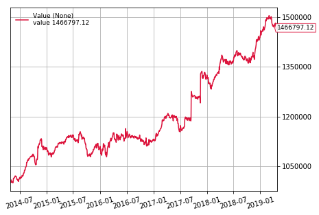
Conclusion

As we can see the algorithm did fairly well! It had a Sharpe ratio of 1.17 with a normalized annual return of 7.9%. Although the returns might not be much better then buying and holding SPY, the volatility is greatly reduced. We do, however, have to take a few things into consideration:

1. The dataset we are using may have a slight survivorship bias as it does not contain companies who where in the S&P 500 5 years ago, but have since been removed.

2. The above backtest assumes that it will compute weights at market close then be able to trade at the exact market close price. In reality we wouldn’t be able to compute weights with the exact close price, but it would be pretty close.

3. Since this particular algorithm trades every stock in the universe at once, the investor will need a large amount of capitol to accurately match the computed weights.