Beating the Odds: Machine Learning for Horse Racing
Published 2019-12-01
Inspired by the story of Bill Benter, a gambler who developed a computer model that made him close to a billion dollars (Chellel, 2018) betting on horse races in the Hong Kong Jockey Club (HKJC), I set out to see if I could use machine learning to identify inefficiencies in horse racing wagering.
Data
The Hong Kong Jockey Club publishes all of the results for each race on their website. I created a script to scrape result cards from all of the historical available races. After running the script I was left with a dataset of 938 races spanning 14 months.
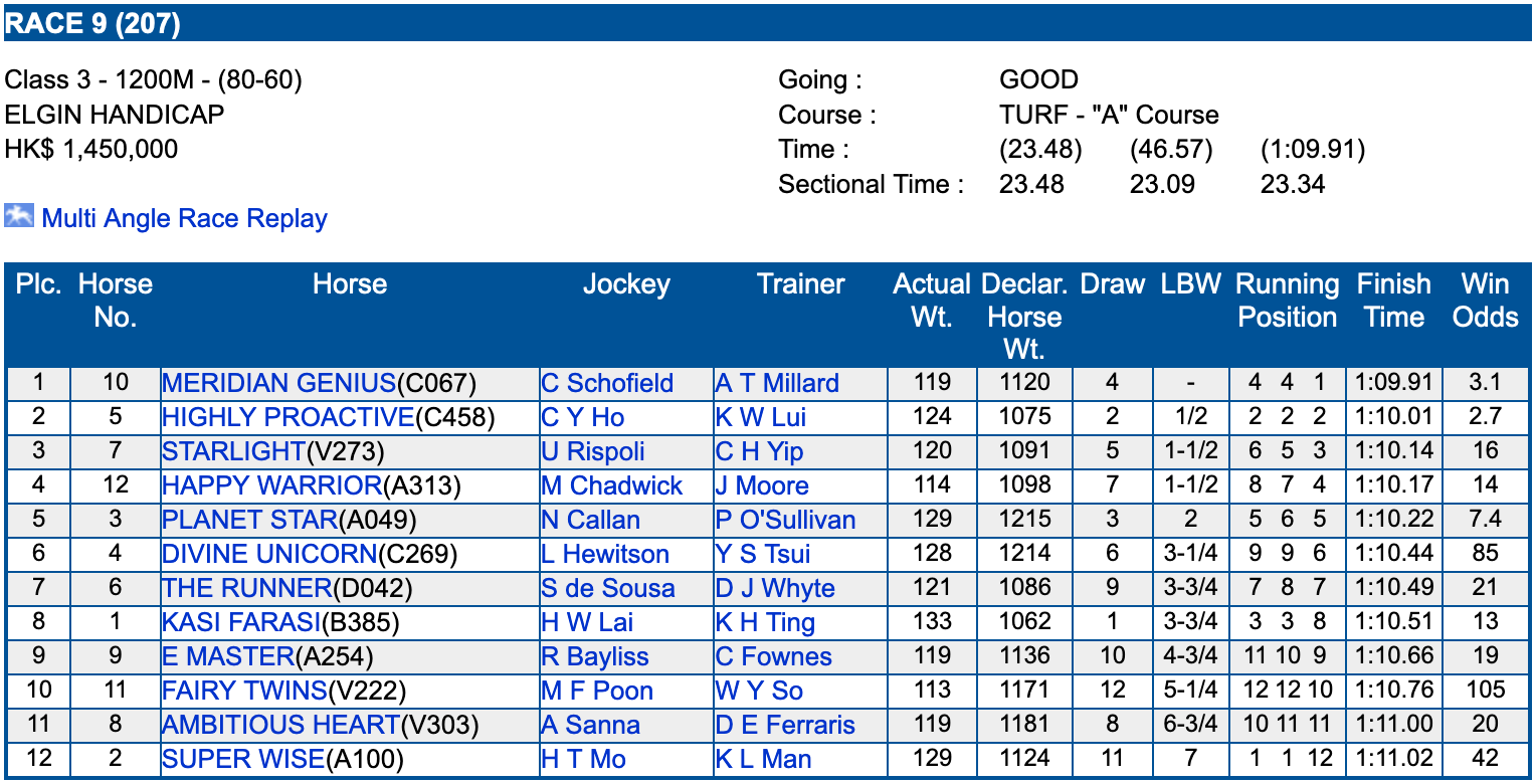 Result card from a HKJC race.
Feature Engineering
Going into this project, I had no industry knowledge about horse racing. Since not much information is provided with the race result cards, much work must be done in engineering and selecting features in order to give a model more predictive power. Listed below are the features being used.
Draw: Which gate the horse starts in. This is randomly assigned before the race. Horses starting closer to the inside of the track (draw 1) generally perform slightly better.
Horse Win Percent: Horse’s win percent over the past 5 races.
Jockey Win Percent: Jockey’s win percent over the past 5 races.
Trainer Win Percent: Trainer’s win percent over the past 5 races.
Actual Weight: How much weight the horse is carrying (jockey + equipment).
Declared Weight: Weight of the horse.
Days Since Last Race: How many days it has been since the horse has last raced. A horse that had been injured in its last race may have not raced recently.
Mean Beyer Speed Figure: Originally introduced in Picking Winners (Beyer, 1994), the Beyer Speed Figure is system for rating a horse’s performance in a race that is comparable across different tracks, distances, and going (track conditions). This provides a way to compare horses that have not raced under the same circumstances. After reading Beyer’s book, I implemented his rating system on my data. For this feature, I calculated the mean speed figure over the horse’s past 5 races.
Last Figure: Speed figure of the last race the horse was in.
Best Figure at Distance: Best speed figure the horse has gotten at the distance of the current race.
Best Figure at Going: Best speed figure the horse has gotten at the track conditions of the current race.
Best Figure at Track: Best speed figure the horse has gotten at the track of the current race.
Engineering more features may yield better results; Benter’s model (Benter, 2008) included many different types of features from many data sources.
Model
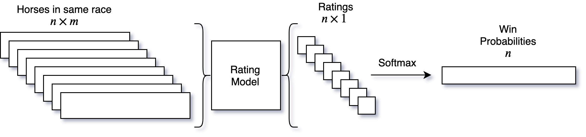
Before creating the model, it is important to understand the goal of the model. In order to not lose money at the race track, one must have an advantage over the gambling public. To do this we need a way of producing odds that are more accurate than public odds. For example, imagine the payout of horse is 5 to 1, and we have a model that indicates the horse’s probability of winning is 0.2, or odds of 4 to 1. Assuming our model is faithful, we would have an edge in this case, as we would be getting an expected return of $(0.2 * (5 + 1)) - 1 = 0.2$ or 20%. How do we create such a model?
Let’s first assume the existence of a function $R$ that provides a rating $R_h$ of a horse $h$, given input features $x_h \in \R^m$:
\[R_h = R(x_h)\]Assuming a horse with a higher rating has a higher probability of winning, we can compute the estimated probability of horse $h$ winning, $\hat{p}_h$, given the ratings of all of the horses in the race:
\[\hat{p}_h = \frac{\exp(R_h)}{\sum_i \exp(R_i)}\]Here we use the softmax function, as its outputs will always sum to 1,
and maintain the same order as the input.
Now that we know how we’ll compute our probabilities, we must define our
rating function $R$. For this we will use a neural network that takes an
input vector of length $m$ (where $m$ is the number of features), and
outputs a single scalar value. The structure of this network consists of
two Fully Connected layers, each followed by a ReLU,
Batch Normalization and Dropout layer. Lastly, there is a final
fully connected layer to produce the single output.
Now we can visualize our model:
Training
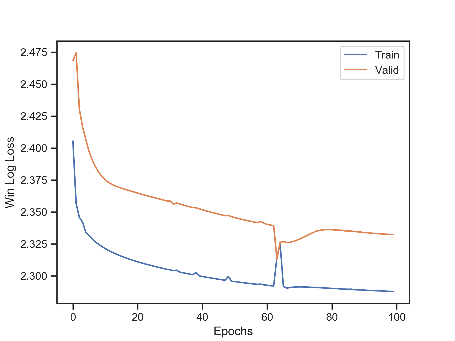
We have defined our model, but how do we train it? For each race, let’s call the winning horse $w$. If we had a perfect model, the predicted probability of $w$ winning should be 1, that is $\hat{p}_w = 1$. We can encourage the model to approach this value by defining a loss function I’ll call win-log-loss:
\[L(\hat{p}_w) = -\log(\hat{p}_w)\]Win-log-loss will approaches 0 as the win-probability of the winner approaches 1, and approaches $\infty$ as the win-probability of the winner approaches 0. Now by minimizing win-log-loss via stochastic gradient descent, we can optimize the predictive ability of our model.
It is important to mention that this method is different than a binary classification. Since the ratings for each horse in a race are calculated using a shared rating network and then converted to probabilities with softmax, we simultaneously reward a high rating from the winner while penalizing high ratings from the losers. This technique is similar to a Siamese Neural Network, which is often used for facial recognition.
Betting
Now that we have predicted win probabilities for each horse in the race we must come up with a method of placing bets on horses. We can compute our own private odds for each horse using $1/\hat{p} - 1$. Now we could just bet on every horse whose odds exceed our private odds, but this may lead to betting on horses with a very low chance of winning. To prevent this, we will only bet on horses whose odds exceed our private odds, and whose odds are less then a certain threshold, which we will find the optimal value of over on our validation set.
Results
We split the scraped race data chronologically into a training, validation, and test set, ensuring there would be no lookahead-bias. We then fit the horse-rating model to our training set, checking its generalization to the validation set:
After fitting the model, we find the optimal betting threshold on the
validation set, in this case odds of 4.9. We can now display our
simulated results of betting 10 dollars on each horse that our model
indicates. To compare, we also show the results of betting 10 dollars
every race on the horse with the best odds, and one of the best
strategies there is, not betting at all.
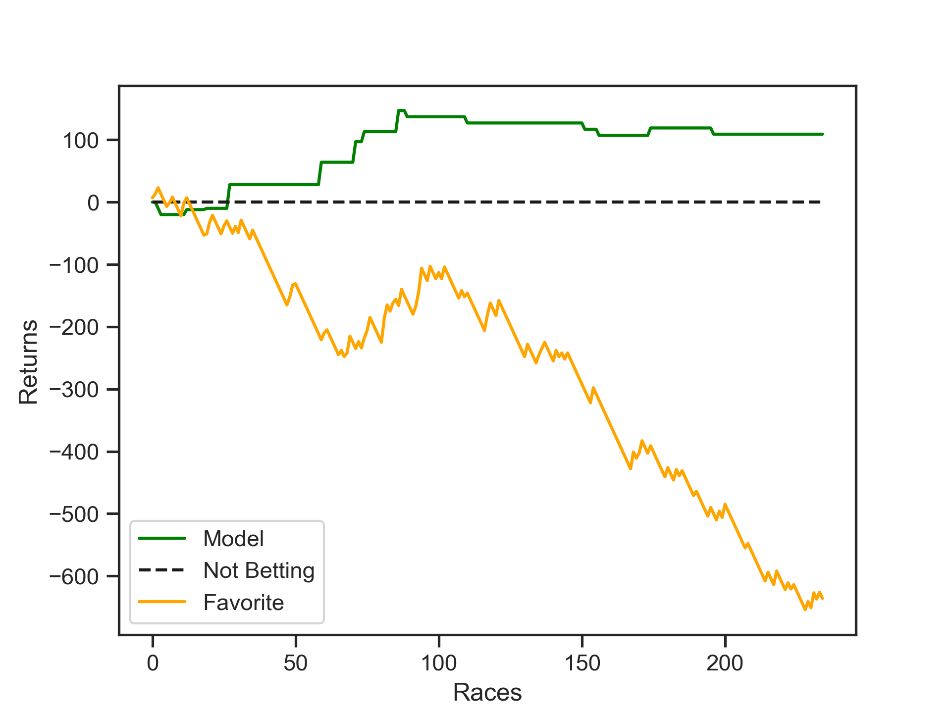
We can see that always betting on the horse with the best odds is a sure-fire way to lose all your money. While the model was profitable over both the training and validation sets, it is hard to say for sure how reliable it is because of the very low frequency of its betting.
Benter claimed that his era was a “Golden Age” for computer betting systems, where computer technology had only recently become affordable and powerful enough to implement such systems. Today, the betting market has likely become much more efficient with large numbers of computer handicappers and more detailed information available to the public. Nevertheless, developing a profitable model, especially with modern machine learning methods, may be a feasible task.
- Chellel, K. (2018). The Gambler Who Cracked the Horse-Racing Code. https://www.bloomberg.com/news/features/2018-05-03/the-gambler-who-cracked-the-horse-racing-code
- Beyer, A. (1994). Picking Winners: A Horseplayer’s Guide. Houghton Mifflin Harcourt.
- Benter, W. (2008). Computer based horse race handicapping and wagering systems: A report. In Efficiency of racetrack betting markets (pp. 183–198). World Scientific.