Performers: The Kernel Trick, Random Fourier Features, and Attention

Published 2020-11-11

Google AI recently released a paper, Rethinking Attention with Performers (Choromanski et al., 2020), which introduces Performer, a Transformer architecture which estimates the full-rank-attention mechanism using orthogonal random features to approximate the softmax kernel with linear space and time complexity. In this post we will investigate how this works, and how it is useful for the machine learning community.

The Kernel Trick

Before we talk about Attention, it is important to understand the kernel trick. Gregory Gundersen gives a great explanation on his blog, but we will go over a brief summary here. This section is not completely necessary for understanding Performers, but might provide some helpful context.

Say we have some data $x \in \mathbb{R}^2$:

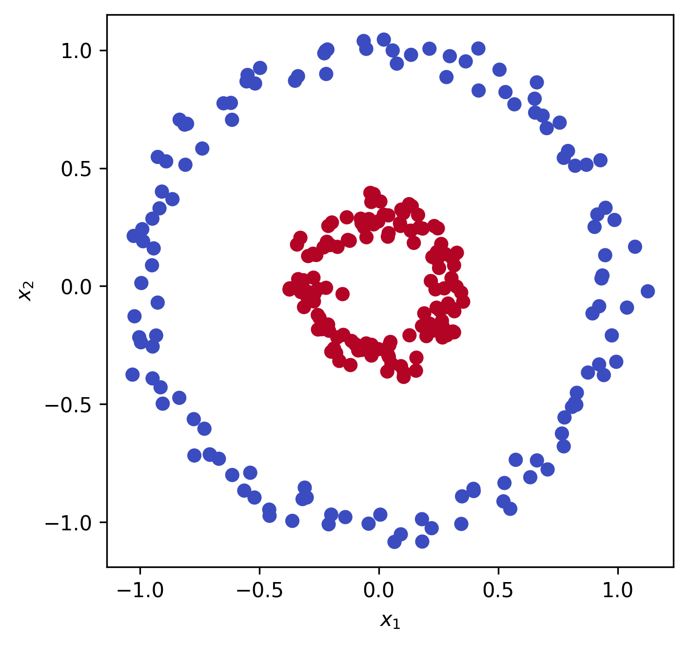
We can see that this data is not linearly separable, i.e. if we wanted to fit a logistic regression or linear support vector machine (SVM) to the data we wouldn’t be able to. How do we get around this? We can map the data into a higher dimension, say $\mathbb{R}^3$, using a function $\varphi : \mathbb{R}^2 \mapsto \mathbb{R}^3$:

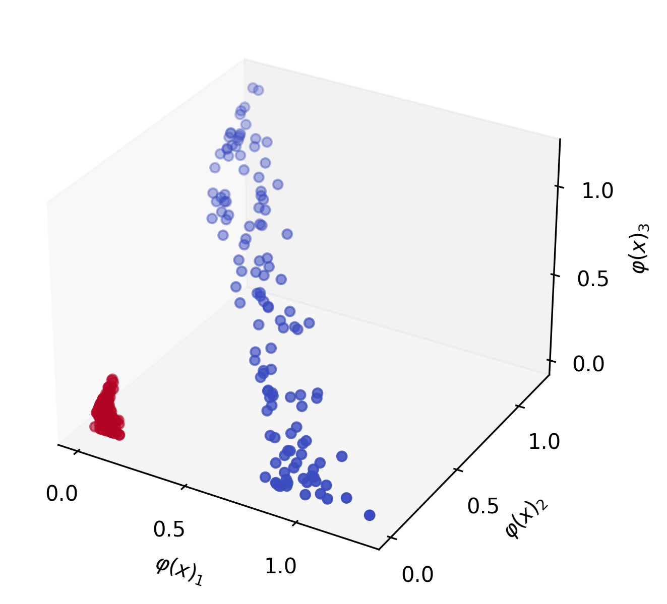
This function $\varphi$ is known as the polynomial kernel of degree $d=2$. If we apply it to our data, $x$, we can visualize that it becomes linearly separable:

Now we can recall the expression for fitting a linear SVM:

Don’t worry if this expression is unfamiliar, just note that we are computing a dot product between two samples $\textcolor{blue}{x_i^\top x_j}$, and repeating this process many times. If we want to use our kernel function $\varphi$ so that the data is linearly seperable, we can simple wrap each $x_n$ with $\varphi$ to map it into a higher dimension:

Now we could stop here, but we can make this more efficient. What we have so far requires computing $\varphi(x_n)$, $N$ times, and the dot-product $\varphi(x_i)^\top \varphi(x_j)$, $N^2$ times, which could start becoming very computationally expensive, especially with kernel functions that map to very high dimensions. How do we get around this? This is where the kernel trick comes in. Suppose we had a function $K : \mathbb{R}^2 \times \mathbb{R}^2 \mapsto \mathbb{R}$ where:

If we can find a $K$ that performs this operation in a lower dimensional space, we can save potentially great amounts of compute. For the polynomial kernel $\varphi$ defined above, finding $K$ is fairly straight forward (derivation is left as an exercise to the reader):

We are now doing the dot-product in lower dimensional space, but we will get the same result as performing the dot-product after the projection. This means we can rewrite our linear SVM expression one more time:

Now instead of doing a dot product in $\mathbb{R}^3$, we are doing it in $\mathbb{R}^2$. This might not make much of an impact in terms of computational cost in this case, but it can make a much bigger difference with more complex kernel functions and higher dimensional data. Next, we will see how Random Fourier Features can reduce the computational cost of some kernel functions even more.

Random Fourier Features

In Random Features for Large-Scale Kernel Machines (Rahimi & Recht, 2007) (which won the NIPS “Test of Time” award in 2017, ten years after it was published), they set out to approximate $K$ using a randomized feature map $z: \mathbb{R}^L \mapsto \mathbb{R}^R$:

Specifically, they prove theoretically that the Gaussian or RBF kernel:

Can be approximated by sampling $z$ from the Fourier transformation. Concretely, one way we can write this as is:

Where $\omega \sim \mathcal{N}_ R(0, I) $ is sampled from a spherical Gaussian. With this approximation, the dot-product no longer needs to be performed in $\mathbb{R}^L$ space, it can now be performed in $\mathbb{R}^R$ space, where $R \ll L$. How is this useful? Using Random Fourier Features, we can approximate any function $K$ that can be written in terms of $K_\text{gauss}$.

Attention

In a previous blog post, we went over the self-attention mechanism, an how it was introduced for language translation. Nowadays, most language models use scaled-dot-product attention as defined in the Transformers paper (Vaswani et al., 2017):

Where $Q, K, V \in \mathbb{R}^{L \times d}$, $L$ is the sequence length, and $d$ is some hidden dimension. We can expand the $\text{softmax}$ and rewrite the expression as the following:

Where $1_L$ is a vector of ones of length $L$. In Python this looks like:

def attention(q, k, v):
    l, d = q.shape
    a = np.exp(q @ k.T * (d ** -0.5))
    d_inv = np.diag(1 / (a @ np.ones(l)))
    return d_inv @ a @ v

This $\text{Attention}$ method has some limitations however; if we examine the attention matrix, $A$, we will realize it is of shape $\mathbb{R}^{L \times L}$, meaning that any operation performed with $A$ will have a time and space complexity that grows quadratically with respect to the sequence length $L$. This puts a limitation on the maximum sequence length that can be used with the Transformer, which means they are not usable for many tasks that may require much longer sequence lengths, such as dialog, protein sequences, and images.

Over the past few months, many have developed their own “X-former” to reduce this complexity, and this is becoming a growing area of research; for a full survey see (Tay et al., 2020).

Performer

Softmax Kernel

The Performer (Choromanski et al., 2020) seeks to reduce the complexity of Attention using random Fourier features. Using the equation above, we can factor out the normalization component, $\sqrt{d}$, in the computation of $A$:

As we continue, we will assume that this normalization is applied beforehand, so we can rewrite as simply:

Now lets say we define a softmax kernel, $K_\text{softmax} : \mathbb{R}^d \times \mathbb{R}^d \mapsto \mathbb{R}$ as:

Using this softmax kernel, we can rewrite the computation of any element within $A$:

Where $q_i$, $k_j$, represent the $i^\text{th}$, $j^\text{th}$ row vector in $Q$, $K$, respectively.

Since the attention matrix is now written as the output of a kernel function $K_\text{softmax}$, we could potentially approximate it at a lower dimensionality as we did for the Gaussian kernel above feature mapping $z: \mathbb{R}^L \mapsto \mathbb{R}^R$:

Note: (Choromanski et al., 2020) uses $\varphi$ to denote this random feature mapping, I am using $z$ for consistency. Working from the definition of the Gaussian kernel function, we can derive $K_\text{softmax}$ in terms of $K_\text{gauss}$:

See Appendix for full derivation. With this derivation, we can come up with our random feature mapping $z_\omega$ that approximates the $K_\text{softmax}$ kernel using the Random Fourier features approximation of the Gaussian kernel:

Where, again, $\omega \sim \mathcal{N}_R(0, I)$ is sampled from a spherical Gaussian. Now, instead of our attention matrix $A$ being of size $\mathbb{R}^{L \times L}$, it is only of size $\mathbb{R}^{R \times L}$, with the sum of each row approximating that of it’s full-rank counterpart.

This looks quite complex at this point, but we can now write the full approximated attention mechanism, $\widehat{\text{Attention}}(Q, K, V)$, in Python like so:

def z_sin_cos(x, omega):
    sin = lambda x: np.sin(2 * np.pi * x)
    cos = lambda x: np.cos(2 * np.pi * x)

    coef = np.exp(np.square(x).sum(axis=-1, keepdims=True) / 2)
    product = np.einsum("...d,rd->...r", x, omega)
    return coef * np.concatenate([sin(product), cos(product)], axis=-1)

def attention_hat(q, k, v, random_dim)
    l, d = q.shape
    normalizer = 1 / (d ** 0.25)               # to normalize before multiplication
    omega = np.random.randn(random_dim, d)     # generate i.i.d. gaussian features
    q_prime = z_sin_cos(q * normalizer, omega) # apply feature map z to Q
    k_prime = z_sin_cos(k * normalizer, omega) # apply feature map z to K
    # rest of attention (note the order of operations is changed for efficiency)
    d_inv = np.diag(1 / (q_prime @ (k_prime.T @ np.ones(l))))
    return d_inv @ (q_prime @ (k_prime.T @ v))

Improvements

Before we make any comparisons between our approximate and full-rank attention method, it is import to mention a couple additional improvements that the authors make to much better estimate the full-rank attention: Orthogonal Random Features, and Positive Random Features.

Orthogonal Random Features

The authors prove theoretically that using exactly orthogonal random features can yield an improved estimation over independent and identically distributed (IID) features:

To further reduce the variance of the estimator (so that we can use even smaller number of random features $R$), we entangle different random samples $\omega_1, …, \omega_R$ to be exactly orthogonal. This can be done while maintaining unbiasedness whenever isotropic distributions $D$ are used (i.e. in particular in all kernels we considered so far) by standard Gram-Schmidt renormalization procedure.

See Proof of Theorem 2 in section F.4 of the appendix in (Choromanski et al., 2020) for the proof that orthogonal random features can improve estimation. My code to generate orthogonal Gaussian features using Gram-Schmidt renormalization can be found here.

IID vs. Orthogonal Random Features

Using $L = 1024$, $d = 16$, we will vary the number of random features $R$ and measure the mean-squared-error (MSE) of our estimated attention and the full-rank attention.

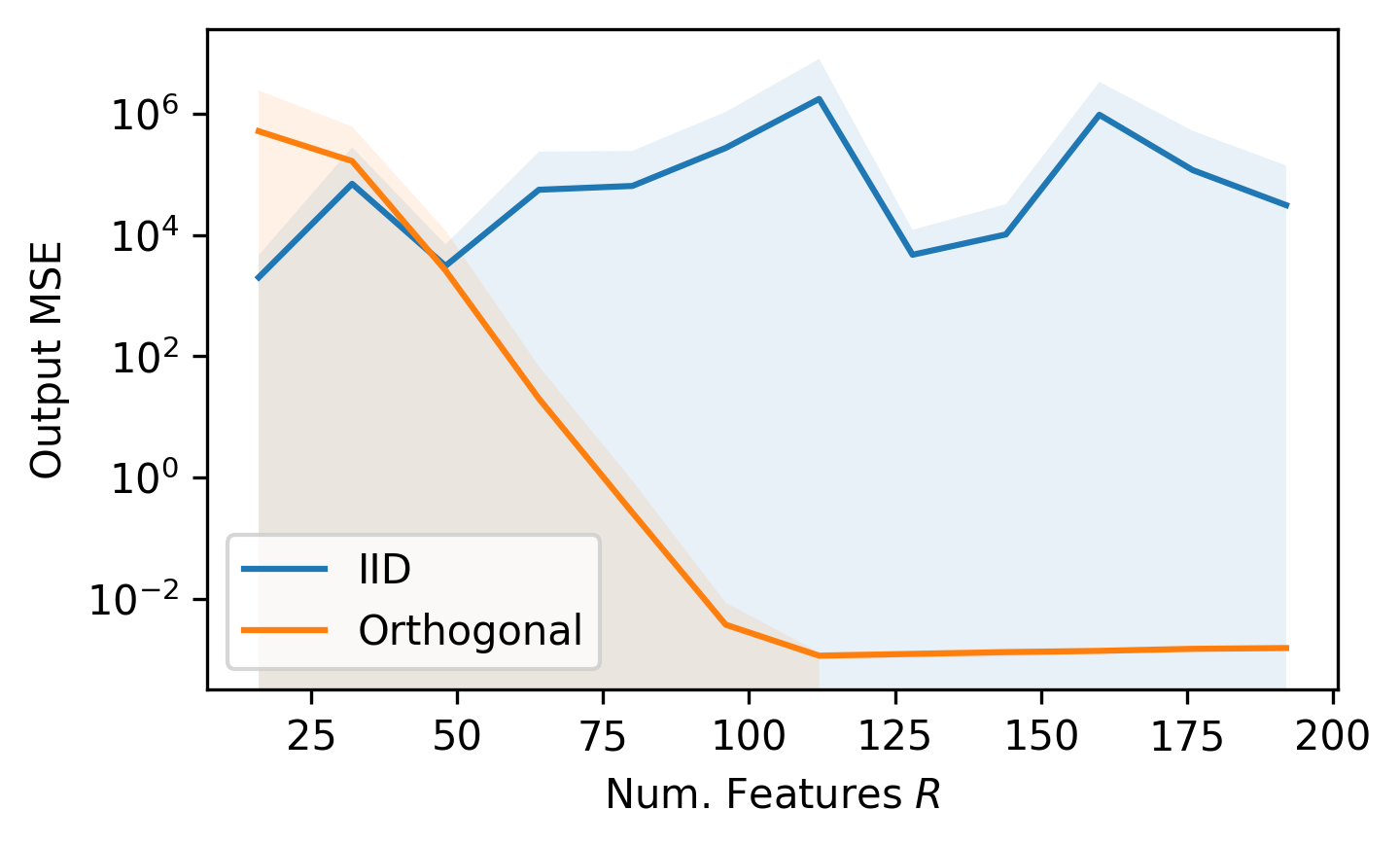
Lines are mean of 15 samples, shaded region is the standard deviation. All of the code to reproduce these figures can be found at: github.com/teddykoker/performer.

We can see that our current approximation method using $z^\text{sin/cos}$ does not work well when using independent and identically distributed (IID) features, but the estimation is quite good for orthogonal random features with a large enough $R$.

Positive Random Features

(Choromanski et al., 2020) also note that the random feature map $z^\text{sin/cos}$ can yield negative values, especially when the kernel outputs approach 0. This is very common for pairs with no interaction, so it can lead to instability in the estimation. To get around this, they propose a new random feature map, $z^\text{positive}$:

Written in Python as:

def z_positive(x, omega):
    coef = np.exp(-np.square(x).sum(axis=-1, keepdims=True) / 2)
    product = np.einsum("...d,rd->...r", x, omega)
    return coef * np.exp(product)

If we compare $z^\text{positive}$ to $z^\text{sin/cos}$, using orthogonal features $\omega$, we can see the improvement:

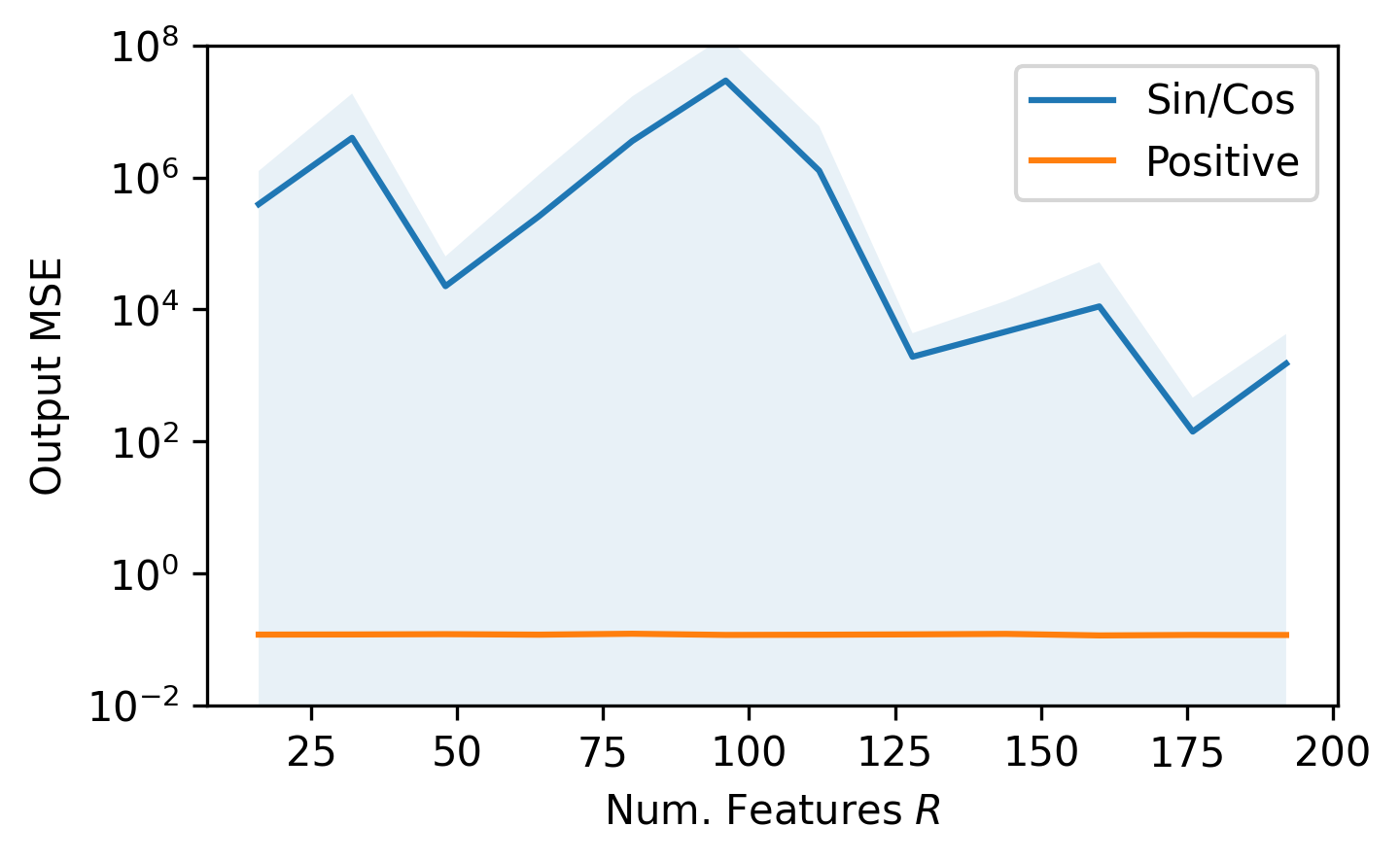
We find that, as was theoretically proven in the paper, the $z^\text{positive}$ feature map with random orthogonal features yields a strong estimation of the full-rank attention mechanism, with a time and space complexity that only grows linearly with respect to sequence length $L$. Ultimately, Performers seem to be a strong approach to reducing the complexity of Transformers, and show potential to be used in many different sub-fields of deep learning.

Acknowledgements

Special thanks to Richard Song of Google AI for providing details around some of the experimentation in the paper.

Appendix

Derive $ K_\text{softmax}(x_i, x_j) = \exp \left( \frac{\lVert x_i \rVert^2}{2} \right) K_\text{gauss}(x_i, x_j) \exp \left( \frac{\lVert x_j \rVert^2}{2} \right) $:

Let $\gamma = \frac{1}{2}$

1. Choromanski, K., Likhosherstov, V., Dohan, D., Song, X., Gane, A., Sarlos, T., Hawkins, P., Davis, J., Mohiuddin, A., Kaiser, L., & others. (2020). Rethinking Attention with Performers. ArXiv Preprint ArXiv:2009.14794.
2. Rahimi, A., & Recht, B. (2007). Random features for large-scale kernel machines. Advances in Neural Information Processing Systems, 20, 1177–1184.
3. Vaswani, A., Shazeer, N., Parmar, N., Uszkoreit, J., Jones, L., Gomez, A. N., Kaiser, Ł., & Polosukhin, I. (2017). Attention is all you need. Advances in Neural Information Processing Systems, 5998–6008.
4. Tay, Y., Dehghani, M., Bahri, D., & Metzler, D. (2020). Efficient transformers: A survey. ArXiv Preprint ArXiv:2009.06732.