Learning to Learn with JAX

Published 2022-04-28

Gradient-descent-based optimizers have long been used as the optimization algorithm of choice for deep learning models. Over the years, various modifications to the basic mini-batch gradient descent have been proposed, such as adding momentum or Nesterov’s Accelerated Gradient (Sutskever et al., 2013), as well as the popular Adam optimizer (Kingma & Ba, 2014). The paper Learning to Learn by Gradient Descent by Gradient Descent (Andrychowicz et al., 2016) demonstrates how the optimizer itself can be replaced with a simple neural network, which can be trained end-to-end. In this post, we will see how JAX, a relatively new Python library for numerical computing, can be used to implement a version of the optimizer introduced in the paper.

The Task: Quadratic Functions

While many tasks can be used, for simplicity and compute we’ll use the Quadratic functions task from the original paper (Andrychowicz et al., 2016):

In particular we consider minimizing functions of the form
\[f(\theta) = \lVert W\theta -y \rVert^2_2\]
for different 10x10 matrices W and 10-dimensional vectors y whose elements are drawn from an IID Gaussian distribution.

Typically you would optimize parameters $\theta$, by repeatedly updating them with some values, $g_t$, obtained by your optimizer:

\[\theta_{t+1} = \theta_t + g_t\]

The optimizer, $g(\cdot)$ will usually computes this update using the gradients $\nabla f(\theta)$, as well as potentially some state, $h_t$:

\[[g_t, h_{t+1}] = g(\nabla f(\theta_t), h_t)\]

SGD

In the case of stochastic gradient descent (SGD), this function is very simple, with no state necessary; the update is computed simply as the negative product of the gradient and the learning rate, $\alpha$ in this case:

\[g_t = - \alpha \cdot \nabla f(\theta_t)\]

In Python we could write this as:

learning_rate = 1.0
def sgd(gradients, state):
    return -learning_rate * gradients, state

We’ll see that the state variable is not modified, but we’ll keep it to be consistent with our framework. Note: learning rates have been searched over log-space for optimal final loss.

Now that we have our framework for optimization defined, we can implement it with JAX:

def quadratic_task(w, y, theta, opt_fn, opt_state, steps=100):
    @jax.jit
    def f(theta):
        product = jax.vmap(jnp.matmul)(w, theta)
        return jnp.mean(jnp.sum((product - y) ** 2, axis=1))

    losses = []
    for _ in range(steps):
        loss, grads = jax.value_and_grad(f)(theta)
        updates, opt_state = opt_fn(grads, opt_state)
        theta += updates
        losses.append(loss)

    return jnp.stack(losses), theta, opt_state

quadratic_task takes our three variables $w$, $y$, and $\theta$, as well as an optimizer function, opt_fn() and opt_state. The gradients of function f() are computed, then passed to the opt_fn(), which then produces the updates and the next state.

There are a couple JAX specific things going on:

jax.vmap(jnp.matmul) performs the matrix multiply operation, automatically vectorizing over the batch dimension
jax.value_and_grad computes the output of a function along with the gradient of that output with respect to its input.
@jax.jit will perform a just-in-time compilation of the function it is wrapping using the XLA compiler, which will optimizer the code for whatever device you are using.

We can see this in action by generating a dataset of $w$, $y$, and $\theta$, and optimizing $\theta$ with the sgd function we defined above:

batch_size = 128
rng = random.PRNGKey(0)
keys = random.split(rng, 3)
w = random.normal(keys[0], (batch_size, 10, 10))
y = random.normal(keys[1], (batch_size, 10))
theta = random.normal(keys[2], (batch_size, 10))

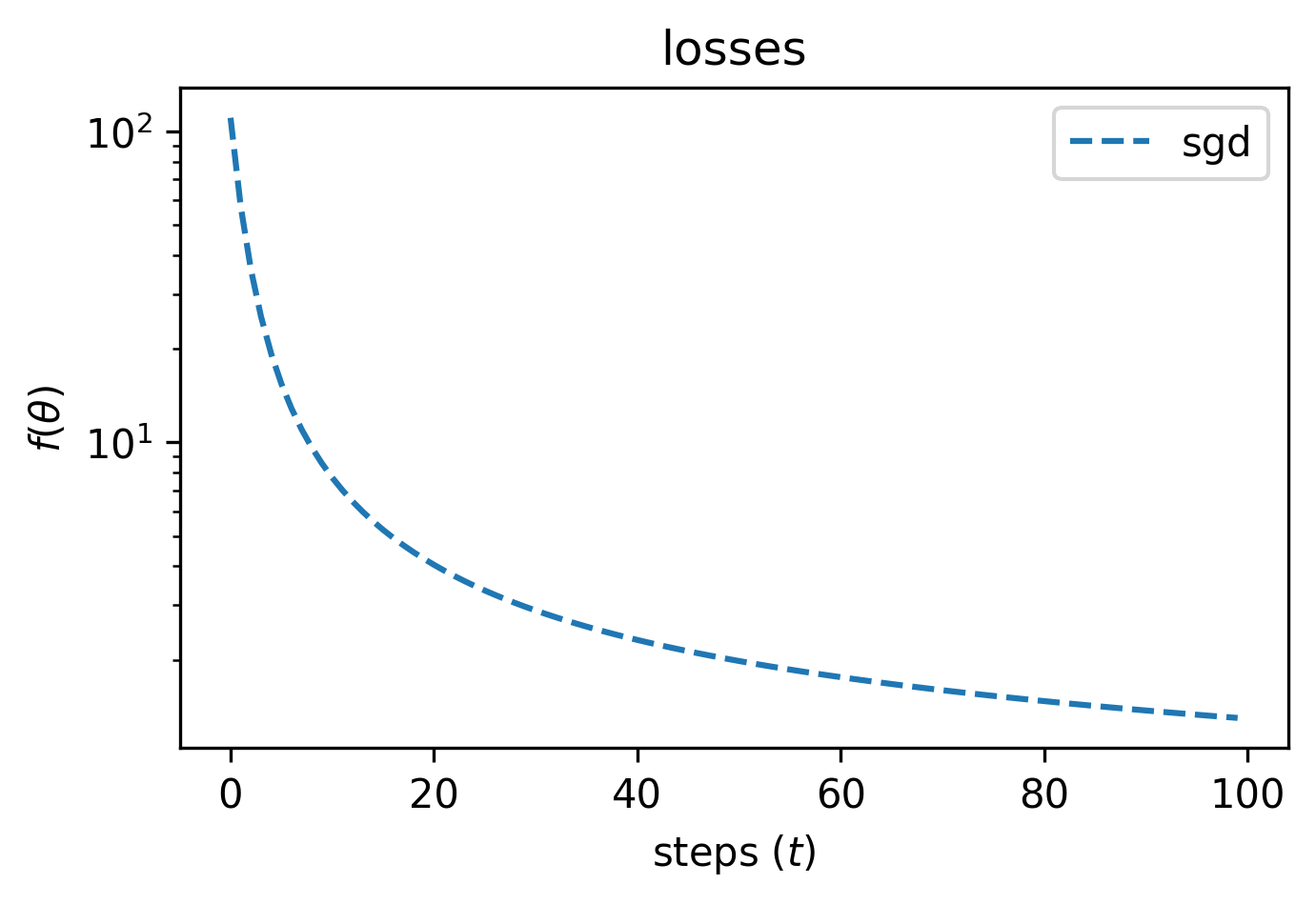
losses, *_ = quadratic_task(w, y, theta, opt_fn=sgd, opt_state=None)

Plotting losses we’ll see that, as expected, $f(\theta)$ is minimized over time:

sgd loss plot

Adam

While simple SGD often works well for gradient-based optimization, Adam (Kingma & Ba, 2014) is another popular choice, which works by maintaining a moving average of the gradient and squared gradient (referred to as the 1st and 2nd moments). While we could implement this ourself, Optax has implemented a JAX version of the optimizer that we can use in a similar manor:

adam = optax.adam(learning_rate=1.0)
losses, *_ = quadratic_task(
    w,
    y,
    theta,
    opt_fn=adam.update,
    opt_state=adam.init(theta),
)

Optax provides a function adam.update(), which will output the next optimizer state $h_{t+1}$ and parameter updates $g_t$, as well as the adam.init() function which will provide the initial state of the optimizer.

We can then plot the losses against losses from SGD.

sgd loss plot

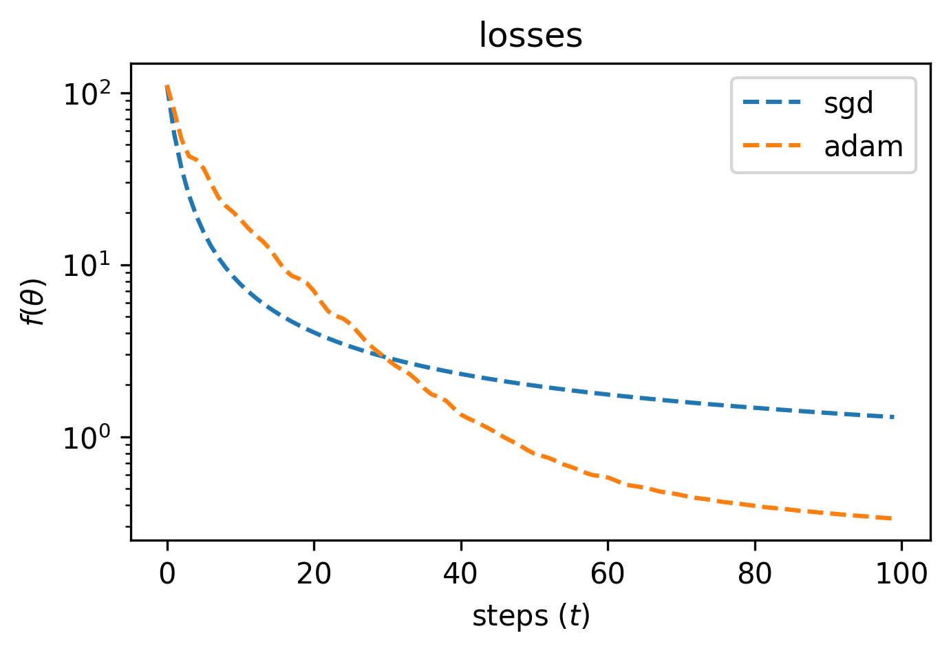
In this case we’ll see that Adam converges faster, and with a lower loss than SGD — but can we do better?

Meta-learning an Optimizer

Looking on back on our formulation for an optimizer:

\[[g_t, h_{t+1}] = g(\nabla f(\theta_t), h_t)\]

We’ll recall that our optimizer function $g(\cdot)$ produces the parameter updates and next state, provided an input and the current state. What kind of neural network does this remind us of? A recurrent one of course! Instead of using an existing optimizer, we can use a recurrent neural network $m(\cdot)$ with its own parameters $\phi$:

\[[g_t, h_{t+1}] = m(\nabla f(\theta_t), h_t, \phi)\]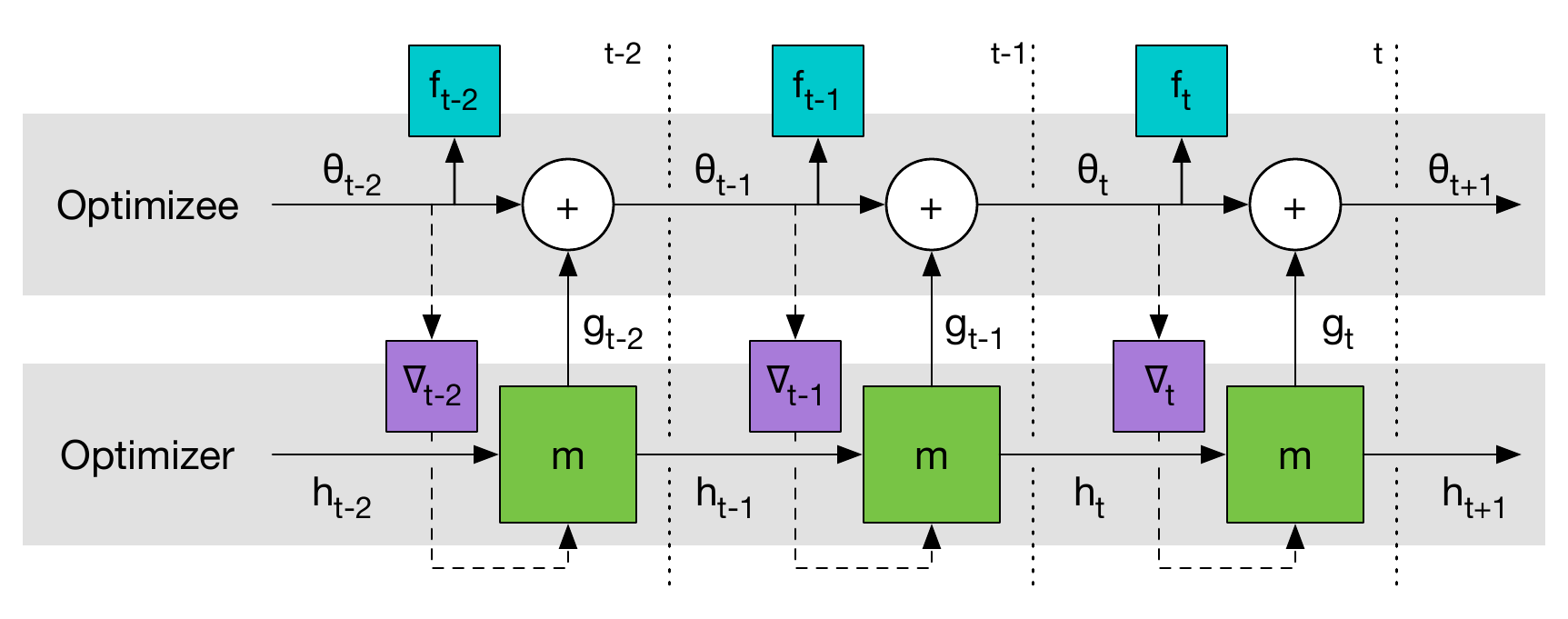

Figure 2. from Learning to Learn by Gradient Descent by Gradient Descent (Andrychowicz et al., 2016). Computational graph used for computing the gradient of the optimizer. Gradients on dashed lines are dropped.

We can implement our own optimizer model as a two-layer LSTM using Flax:

from flax import linen as nn

class LSTMOptimizer(nn.Module):
    hidden_units: int = 20

    def setup(self):
        self.lstm1 = nn.recurrent.LSTMCell()
        self.lstm2 = nn.recurrent.LSTMCell()
        self.fc = nn.Dense(1)

    def __call__(self, gradient, state):
        # gradients of optimizee do not depend on optimizer
        gradient = jax.lax.stop_gradient(gradient)

        # expand parameter dimension to extra batch dimension so that network
        # is "coodinatewise"
        gradient = gradient[..., None]

        carry1, carry2 = state
        carry1, x = self.lstm1(carry1, gradient)
        carry2, x = self.lstm2(carry2, x)
        update = self.fc(x)
        update = update[..., 0]  # remove last dimension
        return update, (carry1, carry2)

    def init_state(self, rng, params):
        return (
            nn.LSTMCell.initialize_carry(rng, params.shape, self.hidden_units),
            nn.LSTMCell.initialize_carry(rng, params.shape, self.hidden_units),
        )

With the optimizer model established, we must now figure out how to train it. We can define a “meta-loss”, which we define as the expected sum of all of the inner losses:

\[\mathcal{L}(\phi) = \mathbb{E}\left[\sum_t f(\theta_t)\right]\]

In this way, if a model is to achieve a small $\mathcal{L}(\phi)$, it must minimize $f(\theta_t)$ as much and as quickly as possible. The meta-model’s parameters $\phi$ can then be optimized with $\nabla \mathcal{L}(\phi)$, which is luckily easy to compute with JAX. First we must initialize our model:

# example gradients of theta
example_input = jnp.zeros((batch_size, 10))

lstm_opt = LSTMOptimizer()
lstm_state = lstm_opt.init_state(rng, example_input)
params = lstm_opt.init(rng, example_input, lstm_state)

Then we define our meta-optimizer, i.e. the optimizer we are using to optimize the optimizer. In this case we’ll use Adam:

meta_opt = optax.adam(learning_rate=0.01)
meta_opt_state = meta_opt.init(params)

Next, we’ll define a single train step, which will train 20 steps of the original quadratic task, using the LSTM model as the optimizer. Although we will eventually optimize for the full 100 steps, we will train over shorter subsequences (effectively truncated backprogagation through time) for stability.

@jax.jit
def train_step(params, w, y, theta, state):
    def loss_fn(params):
        update = partial(lstm_opt.apply, params)
        losses, theta_, state_ = quadratic_task(w, y, theta, update, state, steps=20)
        return losses.sum(), (theta_, state_)

    (loss, (theta_, state_)), grads = jax.value_and_grad(loss_fn, has_aux=True)(params)
    return loss, grads, theta_, state_

Note that we can simply pass the apply() function of the LSTM as the quadratic tasks’s update function, and then we can compute the gradients of the LSTM’s parameters, params, with respect to the sum of the inner losses. JAX makes it very easy to do this because of its functional nature; doing something like this in PyTorch would be more difficult.

Now all we have to do is repeatedly update to the parameters to the LSTM optimizer using its gradients with the meta-optimizer:

for step in range(1000):
    rng, *keys = jax.random.split(rng, 4)
    w = jax.random.normal(keys[0], (batch_size, 10, 10))
    y = jax.random.normal(keys[1], (batch_size, 10))
    theta = jax.random.normal(keys[2], (batch_size, 10))
    lstm_state = lstm_opt.initialize_carry(rng, theta)

    for unrolls in range(5):
        loss, grads, theta, lstm_state = train_step(params, w, y, theta, lstm_state)
        updates, meta_opt_state = meta_opt.update(grads, meta_opt_state)
        params = optax.apply_updates(params, updates)

For each of the 1000 steps, we randomly sample a new $w$, $y$, and $\theta$. We then perform 5 unrolls, each of which optimizes $\theta$ for 20 steps in the train_step we defined above. For each unroll we use the computed gradients to update the LSTM parameters with the meta-optimizer.

Evaluation

With the LSTM optimizer trained, we can now evaluate it on our original quadratic task, and compare it to SGD, Adam, as well as RMSprop and Nesterov’s accelerated gradient (NAG):

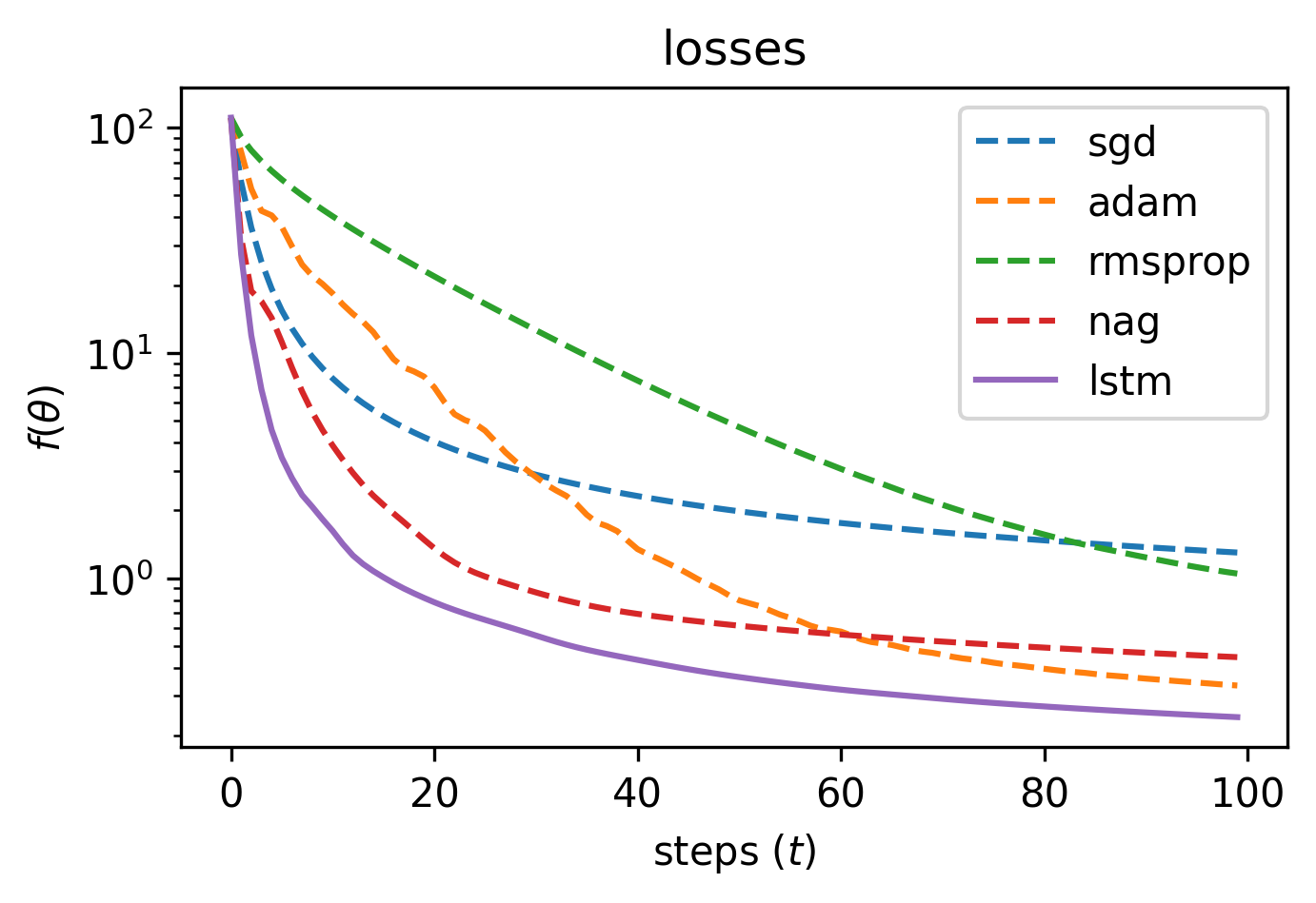
lstm loss plot with other optimizers

Our LSTM optimizer has learned to out-perform the other hand crafted optimizers for the quadratic functions task! The original work goes on to demonstrate training and evaluating the optimizer on other tasks, including MNIST, CIFAR-10, and style transfer, which can be done in the same way we built quadratic_task().

Conclusion

In this post we learned how meta-learned optimizers can be trained via gradient descent, and how to implement one while leveraging JAX as well as other libraries in the JAX ecosystem. A more-organized version of this code including everything to reproduce the figures in this post can be found here:

github.com/teddykoker/learning-to-learn-jax

Sutskever, I., Martens, J., Dahl, G., & Hinton, G. (2013). On the importance of initialization and momentum in deep learning. International Conference on Machine Learning, 1139–1147.
Kingma, D. P., & Ba, J. (2014). Adam: A method for stochastic optimization. ArXiv Preprint ArXiv:1412.6980.
Andrychowicz, M., Denil, M., Gomez, S., Hoffman, M. W., Pfau, D., Schaul, T., Shillingford, B., & De Freitas, N. (2016). Learning to learn by gradient descent by gradient descent. Advances in Neural Information Processing Systems, 29.