Loss Landscapes of Neural Network Wavefunctions

Published 2025-12-10

---

Note: this is condensed version of a project for course 6.7960.

Introduction

Accurate solutions to the Schrödinger equation are essential for modeling the behavior of quantum systems, which is valuable for quantum chemistry and condensed matter physics. However, solving the many-electron Schrödinger equation is notoriously challenging due to the exponential growth of the state space with system size. Traditional numerical methods like coupled cluster (CC) and density functional theory (DFT) make various approximations to manage this complexity, but they often struggle with strongly correlated systems and out-of-equilibrium geometries.

Recent advances in deep learning have opened new possibilities for tackling this challenging problem. Neural quantum Monte Carlo has emerged as a promising approach, using neural networks to approximate wavefunctions while potentially avoiding the exponential computational requirements of exact methods. However, optimizing these neural network wavefunctions poses unique challenges compared to standard deep learning tasks.

In this blog post, we will explore the loss landscape of a simple neural-network wavefunction, investigate why optimization of these neural wavefunctions is difficult, and explore the performance of different optimization methods.

Background

More background and demonstration can be found in my previous post. The time independent Schrödinger equation is given by

\[\hat{H}\psi(\mathbf{X}) = E\psi(\mathbf{X})\]

where $\hat{H}$ is the Hamiltonian operator, wavefunction $\psi(\mathbf{X})$ is an eigenfunction of the system, and $E$ is the energy. The wavefunction is a function of $\mathbf{X} = \left(\mathbf{x}_1, \mathbf{x}_2, …, \mathbf{x}_N \right)$ which are the states of each of the $N$ electrons in a system. Using the Born-Oppenheimer approximation, the Hamiltonian is given by

\[\hat{H} = -\frac{1}{2}\sum_i \nabla^2_i + \sum_{i>j} \frac{1}{|\mathbf{r}_i - \mathbf{r}_j|} - \sum_{iI} \frac{Z_I}{|\mathbf{r}_i - \mathbf{R}_j|} + \sum_{I>J} \frac{Z_I Z_J}{|\mathbf{R}_I - \mathbf{R}_J|}\]

Using the variational principle, we can find the ground state energy of the system by minimizing the following objective:

\[\mathcal{L}(\theta) = \frac{\braket{\psi_\theta|\hat{H}|\psi_\theta}}{\braket{\psi_\theta|\psi_\theta}} = \mathbb{E}_{\mathbf{X}\sim|\psi_\theta|^2} \left[ \frac{\hat{H}\psi_\theta(\mathbf{X})}{\psi_\theta(\mathbf{X})} \right]\]

where the expectation over samples $\mathbf{X}\sim|\psi_\theta|^2$ is obtained through Monte Carlo sampling of the probability distribution defined by the wavefunction using Metropolis-Hastings, a form of Markov Chain Monte Carlo (MCMC).

This optimization presents several unique challenges from a deep learning perspective. Unlike typical supervised learning where gradients can be computed exactly, we must rely on a stochastic estimate of the gradient (Pfau et al., 2020):

\[\nabla_\theta\mathcal{L}(\theta) = 2\mathbb{E}_{\mathbf{X}\sim|\psi_\theta|^2} \left[ \nabla_\theta \log \psi_\theta(\mathbf{X}) \left(\frac{\hat{H}\psi_\theta(\mathbf{X})}{\psi_\theta(\mathbf{X})} - \mathcal{L}(\theta) \right) \right]\]

This stochasticity makes neural wavefunction more difficult to converge to over more traditional deep learning tasks.

Related Work

Several recent works have proposed neural network architectures specifically designed for quantum chemistry applications. FermiNet (Pfau et al., 2020) introduces an architecture that incorporates the physics of fermionic wavefunctions through a novel multi-stream network design that processes single-electron and pair-wise electron features separately. This allows the network to efficiently capture electron-electron correlations while maintaining the required antisymmetry of the wavefunction. Similarly, PauliNet (Hermann et al., 2020) combines deep neural networks with physics-based prior knowledge by incorporating molecular orbitals and explicitly enforcing proper asymptotic behavior. Both approaches demonstrate significant improvements over traditional quantum chemistry methods, particularly for strongly correlated systems. However, these architectures focus primarily on architectural design rather than the optimization challenges that arise during training, which is the focus of this post.

For optimizing of neural wavefunctions, several works have been proposed that build upon standard gradient descent. Methods such as KFAC (Martens & Grosse, 2015) and SPRING (Goldshlager et al., 2024) are second-order optimization methods have been proposed as methods to improve the optimization of neural networks, which we will elaborate on in further detail below in the Methods section.

Lastly, several works such as by (Li et al., 2018) have studied the loss landscapes of neural networks in the context of deep learning. However, this work has been limited to more traditional computer vision and natural language processing tasks.

Methods

Atomic Configuration

In order to study the optimization of neural wavefunctions, we must first define a simple task that can be evaluated fairly quickly with limited computational resources. We choose the Helium atom, which does not have a closed-form solution for the ground-state wavefunction, but has a known exact ground state energy (Zielinski et al., 2005).

We design a simple neural-network wavefunction for the system, which consists of a single Helium atom at the origin with two electrons, $\mathbf{x}_1$ and $\mathbf{x}_2$. We define the wavefunction as:

\[\psi_\theta(\mathbf{x}_1, \mathbf{x}_2) = e^{-2(|\mathbf{r}_1| + |\mathbf{r}_2|)} * \text{MLP}_\theta(|\mathbf{r}_1|, |\mathbf{r}_2|, |\mathbf{r}_1 - \mathbf{r}_2|, \mathbf{r}_1, \mathbf{r}_2)\]

where $\mathbf{r}_i$ and $|\mathbf{r}_i|$ are the displacement and distance of electron $\mathbf{x}_i$ from the nucleus, respectively. The first term is a simple envelope function that ensures the wavefunction decays to zero as electrons move far away from the nucleus, which serves as a good inductive bias for our model. $\text{MLP}_\theta(\cdot)$ is a multi-layer perceptron with parameters $\theta$. For our experiments, it contains three hidden layers of size 32, and a single scalar output. As the wavefunction must be smooth at all points except the cusp, we use the $\tanh$ activation function to enforce this behavior.

Loss Landscapes

To study the loss landscape of the wavefunction, we follow the method introduced by (Li et al., 2018). We sample two random directions, $\sigma$ and $\eta$, that are the same dimensionality as the model weights. Importantly, these model weights must be normalized by the Frobenius norm of each corresponding weight matrix in the trained model. This prevents the scale invariance in network weights from affecting the visualization. Given optimized parameters $\theta^*$, we compute the loss landscape as a function:

\[f(\alpha, \beta) = \mathcal{L}(\theta^* + \alpha\sigma + \beta\eta)\]

Intuitively, this can be viewed as an interpolation between the trained model weights and the random directions.

Natural Gradient Descent and Kronecker-Factored Approximation

Natural gradient descent (Amari, 1998) is a method of optimization that takes into account the curvature of the loss landscape. Given parameters $\theta_t$ at step $t$, the update step is given by

\[\theta_{t+1} = \theta_t - \epsilon \mathbf{F}^{-1} \nabla_\theta \mathcal{L}(\theta_t)\]

where $\epsilon$ is the learning rate. This appears as the standard gradient descent method, with the addition of $\mathbf{F}^{-1}$ which is the inversion of the Fisher information matrix (FIM),

\[\mathbf{F}_{ij} = \mathbb{E}_{\mathbf{X}\sim|\psi_\theta|^2} \left[ \frac{\partial \log \psi_\theta(\mathbf{X})}{\partial \theta_i} \frac{\partial \log \psi_\theta(\mathbf{X})}{\partial \theta_j} \right].\]

This can also be viewed as a form of steepest descent, where the norm is replaced by KL divergence (Amari, 1998). In theory, by leveraging this curvature, we are able to take larger, more informed steps in the parameter space. This is especially useful in our case, where the loss landscape is noisy and has many local minima.

Unfortunately, computing the inverse of the FIM is computationally intractable beyond the smallest of neural networks, as the matrix is of size $n \times n$ for a $n$-parameter model. This is where Kronecker-factored approximate curvature (KFAC) (Martens & Grosse, 2015) comes in.

KFAC makes two key approximations in order to make the computation tractable. First, it assumes that $\mathbf{F}_{ij}$ will be $0$ if parameters $\theta_i$ and $\theta_j$ are not in the same layer. The intuition for this is that parameters from different layers are much less likely to have strong interactions. By making this sparsity assumption the FIM becomes block diagonal, allowing the FIM to be computed layer by layer.

The second approximation is with respect to the calculation of each FIM block. The exact FIM block for a single layer can be written as:

\[\mathbf{F}_{\ell} = \mathbb{E}_{\mathbf{X}\sim|\psi_\theta|^2} \left[ (\mathbf{g}_\ell \otimes \mathbf{a}_\ell) (\mathbf{g}_\ell \otimes \mathbf{a}_\ell)^\top \right]\]

where $\mathbf{g}_\ell$ is the gradient of the loss with respect to the layer output, and $\mathbf{a}_\ell$ is the input to the layer. KFAC leverages the property of the Kronecker product of matrices ${(\mathbf{A} \otimes \mathbf{B})^{-1} = \mathbf{A}^{-1} \otimes \mathbf{B}^{-1}}$ to approximate the inverse of the FIM block as:

\[\mathbf{F}_{\ell}^{-1} \approx \mathbb{E}_{\mathbf{X}\sim|\psi_\theta|^2} \left[\mathbf{g}_\ell \mathbf{g}_\ell^\top \right]^{-1} \otimes \mathbb{E}_{\mathbf{X}\sim|\psi_\theta|^2} \left[\mathbf{a}_\ell \mathbf{a}_\ell^\top \right]^{-1}\]

This further reduces the order of magnitude of computation as the dimensionality of the vectors $\mathbf{g}_\ell$ and $\mathbf{a}_\ell$ will generally be much smaller than that of the model weights. These two approximations will allow us to efficiently compute the natural gradient, which we will use to optimize our wavefunction.

Results

Loss Landscapes

We reimplement the method from (Li et al., 2018) in JAX, using two random directions in the model weight space, normalized by the norm of each weight matrix. To verify our implementation, we first look at the loss landscape of a simple convolutional neural network (CNN) trained on MNIST.

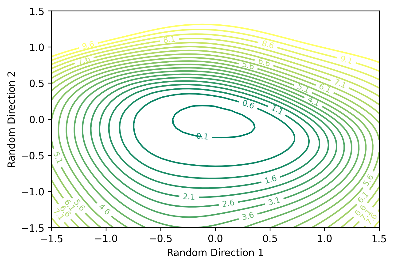
Figure 2: Loss landscape of a CNN neural network trained on MNIST. Contour levels show cross-entropy loss values over the test set.

We observe the loss landscape to appear quite smooth and convex, centered around the optimal parameters. Based on this geometry, it is not surprising that traditional gradient descent methods are able to optimize the network quite well.

With the loss landscape of a CNN in MNIST, we can compare this to the loss landscape of our MLP Helium wavefunction. Since the gradient is computed over an expectation of MCMC samples, we will visualize the landscape under differing numbers of samples to observe the effect of this stochasticity.

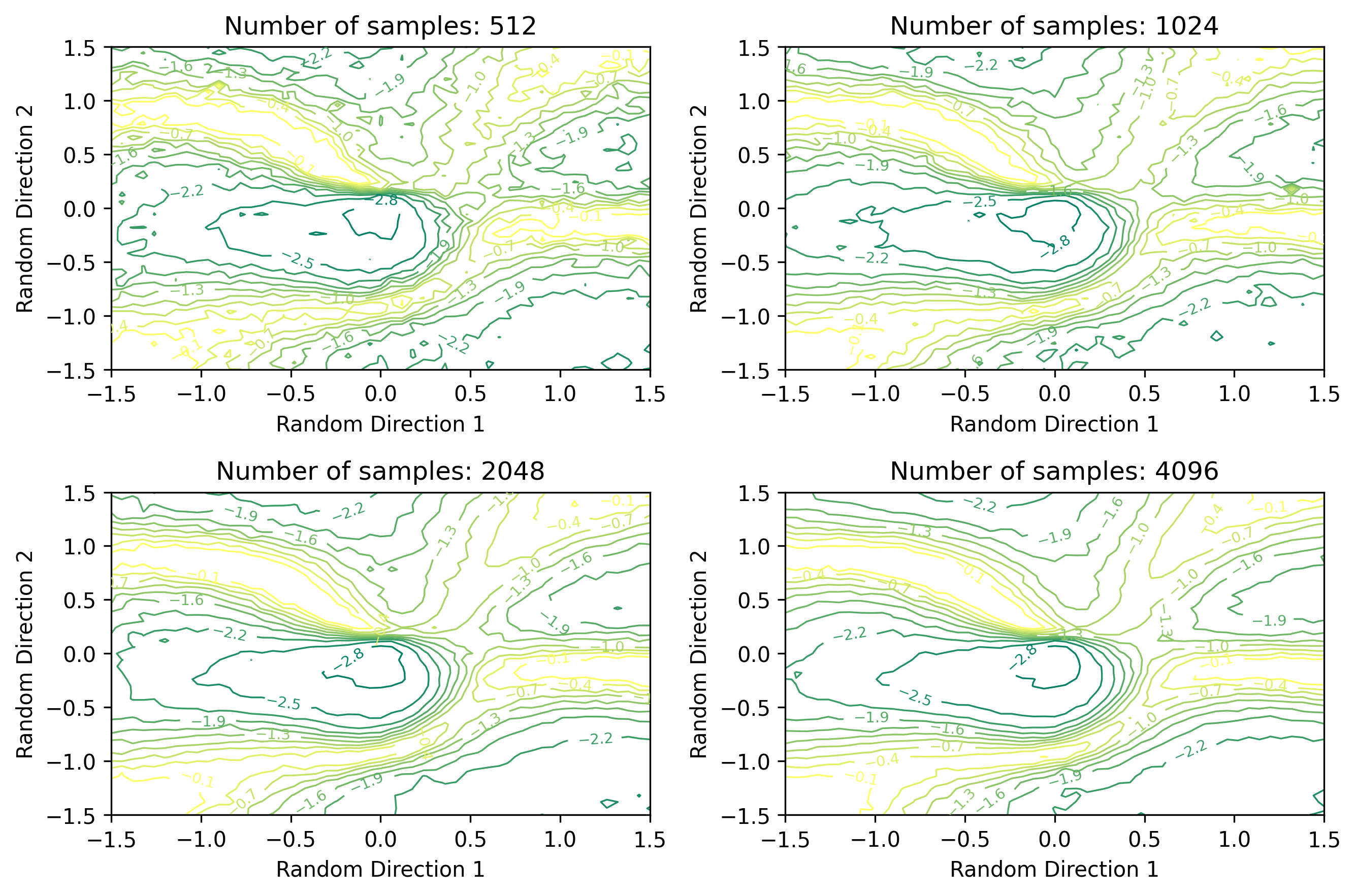
Figure 3: Loss landscape of a three-layer MLP trained to solve the Helium ground state energy. Contour levels show the estimated total energy of the wavefunction in a.u.. Note that the ground state energy of He is approximately -2.9 a.u.., which appears in the center of the landscape. Here we show how the loss landscape changes with 512, 1024, 2048, and 4096 samples.

Compared to the CNN MNIST loss landscape, we observe several factors that likely make optimization of the wavefunction more difficult. First, we observe several local minima appearing as additional valleys in the landscape. These local minima are not as deep as the global minimum (or exact energy), and could therefore cause the optimizer to converge to a suboptimal solution. Next, we observe the loss landscape appears to be quite noisy. With 512 samples, the contour lines appear quite jagged. While the 4096 sample landscape appears somewhat less jagged, the effects of the MCMC sampling are still quite apparent. This jaggedness could cause first-order optimizers to take steps in the wrong direction, causing the optimizer to diverge from the optimal wavefunction. This further motivates the use of second-order methods, such as KFAC.

Optimizers

We use kfac_jax implementation of KFAC to optimize our Helium MLP wavefunction. We note that special care must be taken to register the individual layers of the model, so the layer-wise Kronecker factors can be computed correctly. In addition to KFAC, we evaluate the performance of popular first-order methods SGD, RMSProp (Hinton et al., 2012), and Adam (Kingma & Ba, 2014). With the exception of learning rate, we maintain default hyperparameters for each optimizer. For learning rate we trial values in [3e-3, 1e-2, 3e-2, 1e-1] and choose the learning rate producing the lowest energy after 5000 iterations. This ensures a fair comparison between the optimizers. Here we show the total energy of the wavefunction over training for each optimizer in its optimal setting, comparing to the exact ground state energy of the Helium atom. Note that we use 4096 MCMC samples for the gradient calculation, which we found to have the smoothest loss landscape.

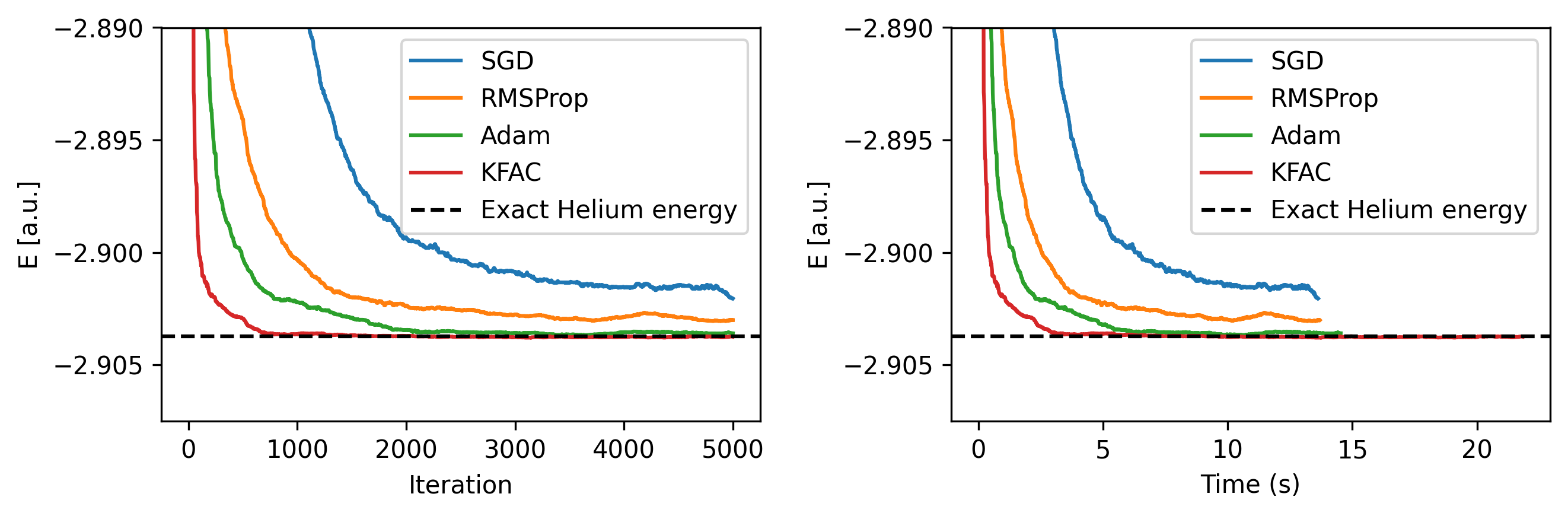
Figure 4: Total energy of wavefunction during training under different optimizers with tuned learning rates. Here the median energy over the last 50 iterations is shown. Training times are shown for a single NVIDIA A5500 GPU.

We find KFAC is able to converge faster than SGD, RMSProp, and Adam, and converges to a lower energy than the other optimizers. Of the first-order methods, Adam shows the best performance, demonstrating why it is often a popular in deep learning optimizers. Since KFAC requires additional computation, we also compare it to the wall-clock time of the other optimizers. Despite the iteration speed being significantly slower, KFAC still converges faster in wall-clock time.

Lastly, we can use our optimized wavefunctions to compute the ground state energy of our system. Using the the last 1000 iterations (of 4096 samples each) we can estimate the total energy to several decimal places, quantifying the standard error through a reblocking procedure (Wolff, 2004).

Optimizer	E (a.u.)
SGD	-2.90166(9)
RMSProp	-2.90289(4)
Adam	-2.90354(3)
KFAC	-2.90372(1)
Exact	-2.90372

Table 1: Ground state energy and standard error of the MLP-based wavefunction using different optimizers. Statistics are computed using a reblocking method (Wolff, 2004), to account for autocorrelation in the MCMC samples.

While each optimizer is able to achieve an energy close to the exact ground state energy, we note that KFAC is the only optimizer that is able to converge to the exact solution within standard error. By the variational principle, achieving the exact ground state energy implies that the neural wavefunction has effectively matched the exact ground state wavefunction, which is desirable for computing exact solutions for other ground state physical properties.

Conclusion

In this work, we investigated the optimization challenges that arise when training neural network wavefunctions. Through visualization of the loss landscape, we demonstrated that optimizing neural wavefunctions involves traversing through a much more complex optimization surface compared to standard deep learning tasks. Not only does the landscape contain multiple local minima, but the stochastic nature of the Monte Carlo gradient estimation introduces significant noise that increases as the number of samples decreases.

Our experiments comparing different optimizers revealed that incorporating curvature information through KFAC’s approximation of natural gradient descent provides substantial benefits. KFAC was the only method to achieve the exact ground state energy within statistical error, despite its higher per-iteration computational cost. This suggests that accounting for the geometry of the parameter space is crucial for finding physically exact solutions in quantum systems, not just for faster convergence.

The full code for this post can be found at github.com/teddykoker/vmc-jax.

---

1. Pfau, D., Spencer, J. S., de G. Matthews, A. G., & Foulkes, W. M. C. (2020). Ab-Initio Solution of the Many-Electron Schrödinger Equation with Deep Neural Networks. Phys. Rev. Research, 2(3), 033429.
2. Hermann, J., Schätzle, Z., & Noé, F. (2020). Deep-neural-network solution of the electronic Schrödinger equation. Nature Chemistry, 12(10), 891–897.
3. Martens, J., & Grosse, R. (2015). Optimizing neural networks with kronecker-factored approximate curvature. International Conference on Machine Learning, 2408–2417.
4. Goldshlager, G., Abrahamsen, N., & Lin, L. (2024). A Kaczmarz-inspired approach to accelerate the optimization of neural network wavefunctions. Journal of Computational Physics, 516, 113351.
5. Li, H., Xu, Z., Taylor, G., Studer, C., & Goldstein, T. (2018). Visualizing the loss landscape of neural nets. Advances in Neural Information Processing Systems, 31.
6. Zielinski, T. J., Harvey, E., Sweeney, R., & Hanson, D. M. (2005). Quantum states of atoms and molecules. ACS Publications.
7. Amari, S.-I. (1998). Natural gradient works efficiently in learning. Neural Computation, 10(2), 251–276.
8. Hinton, G., Srivastava, N., & Swersky, K. (2012). Neural networks for machine learning lecture 6a overview of mini-batch gradient descent.
9. Kingma, D. P., & Ba, J. (2014). Adam: A method for stochastic optimization. ArXiv Preprint ArXiv:1412.6980.
10. Wolff, U. (2004). Monte Carlo errors with less errors. Computer Physics Communications, 156(2), 143–153.