PFT: Phonon Fine-tuning for Machine Learned Interatomic Potentials
Published 2026-02-10
This blog post accompanies our recent paper PFT: Phonon Fine-tuning for Machine Learned Interatomic Potentials. Here we will briefly introduce some of the background for machine learned interatomic potentials (MLIP) and phonons, and then walk through a small example that demonstrates how we developed the approach. The code accompanying the full paper is at atomicarchitects/nequix, while the full demo in this post (in both JAX and PyTorch) can be found at teddykoker/nequix-examples.
Many materials properties depend on higher-order derivatives of the potential energy surface, yet machine learned interatomic potentials trained with a standard loss on energy, force, and stress errors can exhibit error in curvature, degrading the prediction of vibrational properties. We introduce phonon fine-tuning (PFT), which directly supervises second-order force constants of materials by matching MLIP energy Hessians to DFT-computed force constants from finite displacement phonon calculations. To scale to large supercells, PFT stochastically samples Hessian columns and computes the loss with a single Hessian-vector product. We also use a simple co-training scheme to incorporate upstream data to mitigate catastrophic forgetting. On the MDR Phonon benchmark, PFT improves Nequix MP by 55% on average across phonon thermodynamic properties and achieves state-of-the-art accuracy among models trained on Materials Project trajectories. PFT also generalizes to improve properties beyond second-derivatives, improving thermal conductivity predictions that rely on third-order derivatives of the potential energy.
Background
Machine learned interatomic potentials (MLIPs) seek to model the potential energy surface of atomistic systems. That is, given an atomic configuration $\mathbf{r}$, what is the predicted energy $\hat{E}(\mathbf{r})$. This can be useful for running molecular dynamics simulations, structural optimization, and computing physical properties of molecules and materials.
It is common to use a so-called conservative model, where the force on each atom is calculated as the negative gradient of the energy with respect to its position,
\[\hat{\mathbf{F}}_a = -\nabla_{\mathbf{r}_a} \hat{E}(\mathbf{r})\]and the stress upon the system (in the case of periodic boundaries) is computed as the derivative of energy with respect to a strain tensor $\varepsilon$,
\[\hat{\sigma}_{ij} = \frac{1}{V} \frac{\partial \hat{E}(\mathbf{r})}{\partial \varepsilon_{ij}}\bigg\rvert_{\varepsilon=0}\]As the name implies, this ensures that forces are conservative, i.e. the integral of the forces along a path that start and end at the same configuration is 0.
Models are typically trained on the energy, forces, and stress of quantum mechanical calculations such as density functional theory (DFT), using a loss function such as
\[\mathcal{L}_\text{EFS} = \lambda_E\mathcal{L}_E + \lambda_F\mathcal{L}_F + \lambda_\sigma\mathcal{L}_\sigma\]with individual terms for the energy, force, and stress respectively are defined as:
\[\mathcal{L}_E = \left| \frac{\hat{E}}{N_a} - \frac{E}{N_a} \right| \qquad \mathcal{L}_F = \frac{1}{N_a} \sum_{a=1}^{N_a} \left\lVert \hat{\mathbf{F}}_a - \mathbf{F}_{a} \right\rVert_2^2\] \[\mathcal{L}_\sigma = \frac{1}{9} \sum_{i=1}^{3} \sum_{j=1}^{3} \left| \hat{\sigma}_{ij} - \sigma_{ij} \right|\]Each weighted by some coefficient $\lambda$. Here we normalize by the number of atoms, $N_a$.
Phonons and vibrational properties
Phonons are quasiparticles that describe small lattice vibrations around a local minimum of the potential energy surface. The spectra and scattering of phonons describe many materials properties of interest, including thermal conductivity, thermal expansion, heat capacity and dynamic stability.
Phonons are obtained from the eigendecomposition of the dynamical matrix, which is constructed from second-order force constants. These force constants, $\Phi$, are the second derivative, or Hessian of the energy with respect to displacement of two atoms:
\[\Phi_{aibj} = \frac{\partial^2 E}{\partial r_{a,i}\partial r_{b,j}}\]If we view a material as being constructed from atoms connect by strings, the force constants essentially describe the stiffness of those springs.
There are generally two ways do conduct phonon calculations. One is density
functional perturbation theory (DFPT), which directly computes force constants
directly using linear response. Alternatively, finite-displacement can be used,
where force constants are extracted from forces generated by small (typically
0.01 Å) displacements. This is implemented in software such as
phonopy, which was used to generate the data we are using (Loew et al., 2025).
Using phonopy, we can compute the force constants for Silicon
(mp-149), of which we
display the components in the $x$ direction below:
ph_ref = phonopy.load(f"mp-149.yaml")
ph_ref.produce_force_constants()
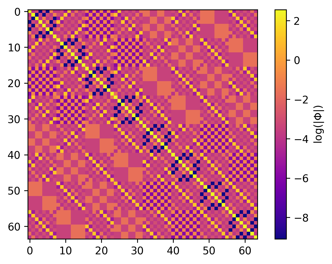
Here we see the $x$-components of the force constants between each of the 64 atoms in the supercell. The supercell looks like:
atoms = ase.Atoms(
    symbols=ph_ref.supercell.symbols,
    positions=ph_ref.supercell.positions,
    cell=ph_ref.supercell.cell,
    pbc=True,
)
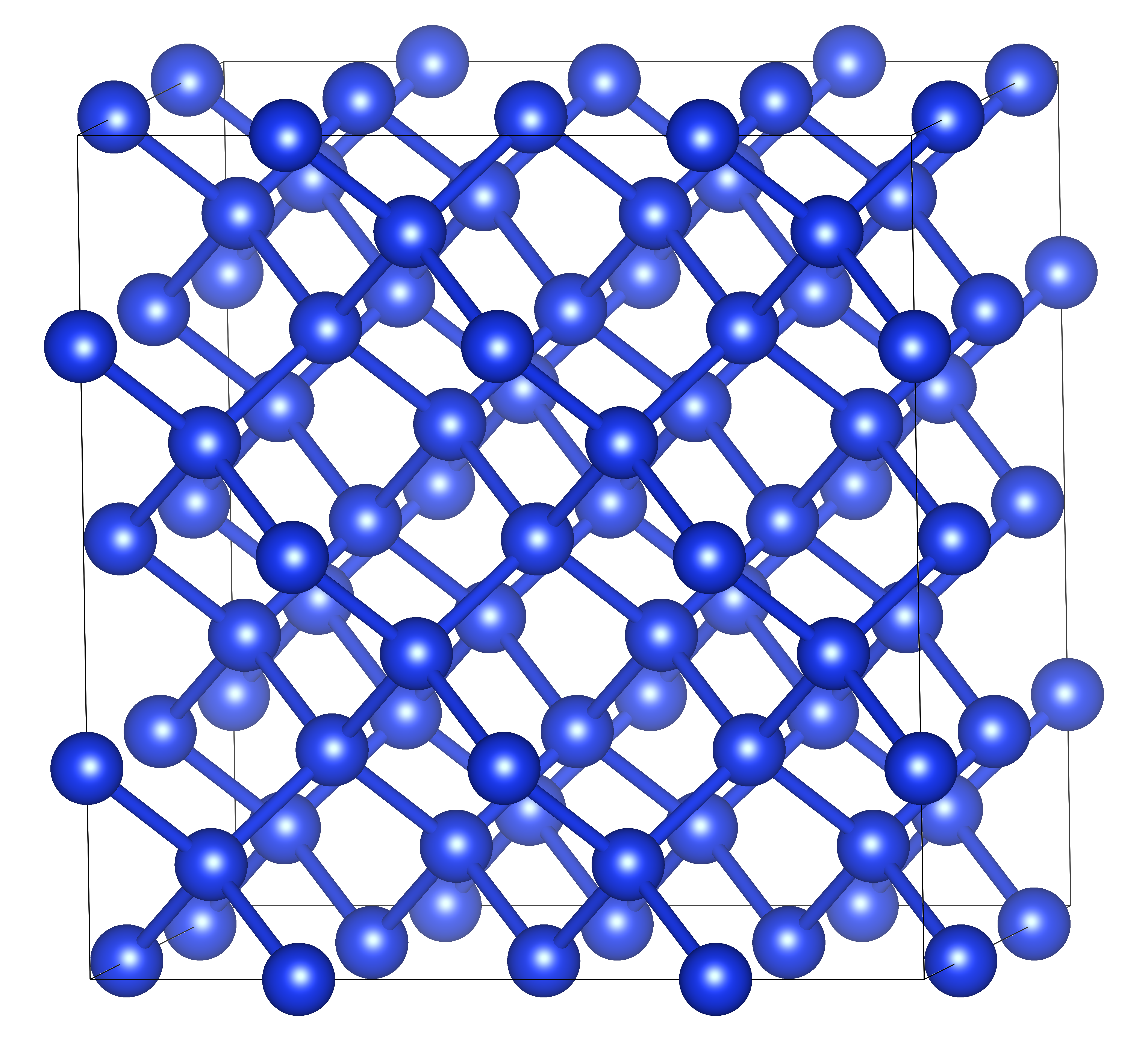
For accurate finite displacement calculations, using a large supercell is necessary to minimize interactions between the displaced atom and periodic copies of itself. This creates a very large Hessian which can be prohibitively expensive to compute analytically, and especially backpropragate through for training. To illustrate this, let’s first try training a small version of the Nequix model (Koker et al., 2025) on the Silicon force constants. We’ll use the same settings as the foundation model, but decrease radial cutoff, the number of layers, and the size of the hidden irreducible representations:
cutoff = 5.0
key = jax.random.key(0)
model = Nequix(
    key=key,
    n_species=1,
    cutoff=cutoff,
    hidden_irreps="32x0e + 32x1o + 32x2e",
    n_layers=3,
    radial_basis_size=8,
    radial_mlp_size=64,
    radial_mlp_layers=2,
)
cutoff = 5.0
device = torch.device("cuda")
model = NequixTorch(
    n_species=1,
    cutoff=cutoff,
    hidden_irreps="32x0e + 32x1o + 32x2e",
    n_layers=3,
    radial_basis_size=8,
    radial_mlp_size=64,
    radial_mlp_layers=2,
).to(device)
Next we prepare the atoms into a graph and flatten our force constants into a $3N\times 3N$ matrix.
atom_indices = atomic_numbers_to_indices(set(atoms.get_atomic_numbers()))
graph = preprocess_graph(atoms, atom_indices, cutoff, targets=False)

# (n, n, 3, 3) -> (3n, 3n)
ref_hessian = (
    jnp.array(ph_ref.force_constants, dtype=jnp.float32)
    .swapaxes(1, 2)
    .reshape(graph["n_node"][0] * 3, graph["n_node"][0] * 3)
)
atom_indices = atomic_numbers_to_indices(set(atoms.get_atomic_numbers()))
g = preprocess_graph(atoms, atom_indices, cutoff, targets=False)
graph = {
    k: torch.as_tensor(
        v, device=device, dtype=torch.float32 if v.dtype == np.float32 else torch.long
    )
    for k, v in g.items()
}

# (n, n, 3, 3) -> (3n, 3n)
ref_hessian = (
    torch.tensor(ph_ref.force_constants, dtype=torch.float32, device=device)
    .swapaxes(1, 2)
    .reshape(g["n_node"][0] * 3, g["n_node"][0] * 3)
)
Training
To train on the force constants, we first define our energy function
$\hat{E}(\mathbf{r})$ or energy_fn(). This is simply the sum of the atom
energies predicted by the model. In order to compute the Hessian, we compute the
Jacobian of the gradient of the energy function. Using the forward-mode Jacobian
(jax.jacfwd or torch.func.jacfwd) over the reverse mode gradient (jax.grad
or torch.func.grad) is generally more efficient. The loss is then simply the
mean absolute error between the Hessian computed from the model and the reference force constants.
def train(model, graph, ref_hessian, n_epochs=200, lr=0.003):
    def energy_fn(model, pos_flat):
        pos = pos_flat.reshape(graph["positions"].shape)
        offset = graph["shifts"] @ graph["cell"]
        disp = pos[graph["senders"]] - pos[graph["receivers"]] + offset
        return model.node_energies(
            disp, graph["species"], graph["senders"], graph["receivers"]
        ).sum()

    grad_fn = jax.grad(energy_fn, argnums=1)

    def hessian_fn(model, x):
        return jax.jacfwd(lambda pos: grad_fn(model, pos))(x)

    optimizer = optax.adam(lr)
    opt_state = optimizer.init(eqx.filter(model, eqx.is_array))

    @eqx.filter_jit
    def train_step(model, opt_state, pos_flat):
        def loss_fn(model):
            hessian = hessian_fn(model, pos_flat)
            return jnp.abs(hessian - ref_hessian).mean()

        loss, grads = eqx.filter_value_and_grad(loss_fn)(model)
        updates, opt_state_new = optimizer.update(grads, opt_state, model)
        model = eqx.apply_updates(model, updates)
        return model, opt_state_new, loss

    pos_flat = graph["positions"].flatten()
    losses = []
    for epoch in tqdm(range(n_epochs)):
        model, opt_state, loss = train_step(model, opt_state, pos_flat)
        losses.append(float(loss))

    return losses
def train(model, graph, ref_hessian, n_epochs=200, lr=0.003):
    def energy_fn(pos_flat):
        pos = pos_flat.view(*graph["positions"].shape)
        offset = graph["shifts"] @ graph["cell"]
        disp = pos[graph["senders"]] - pos[graph["receivers"]] + offset
        return model.node_energies(
            disp, graph["species"], graph["senders"], graph["receivers"]
        ).sum()

    grad_fn = torch.func.grad(energy_fn)
    hessian_fn = torch.compile(torch.func.jacfwd(grad_fn))

    pos_flat = graph["positions"].flatten()
    losses = []
    optimizer = torch.optim.Adam(model.parameters(), lr=lr)


    for epoch in tqdm(range(n_epochs)):
        optimizer.zero_grad()
        hessian = hessian_fn(pos_flat)
        loss = (hessian - ref_hessian).abs().mean()
        loss.backward()
        optimizer.step()
        losses.append(loss.item())

    return losses
We can use this function to train our model, as shown below:
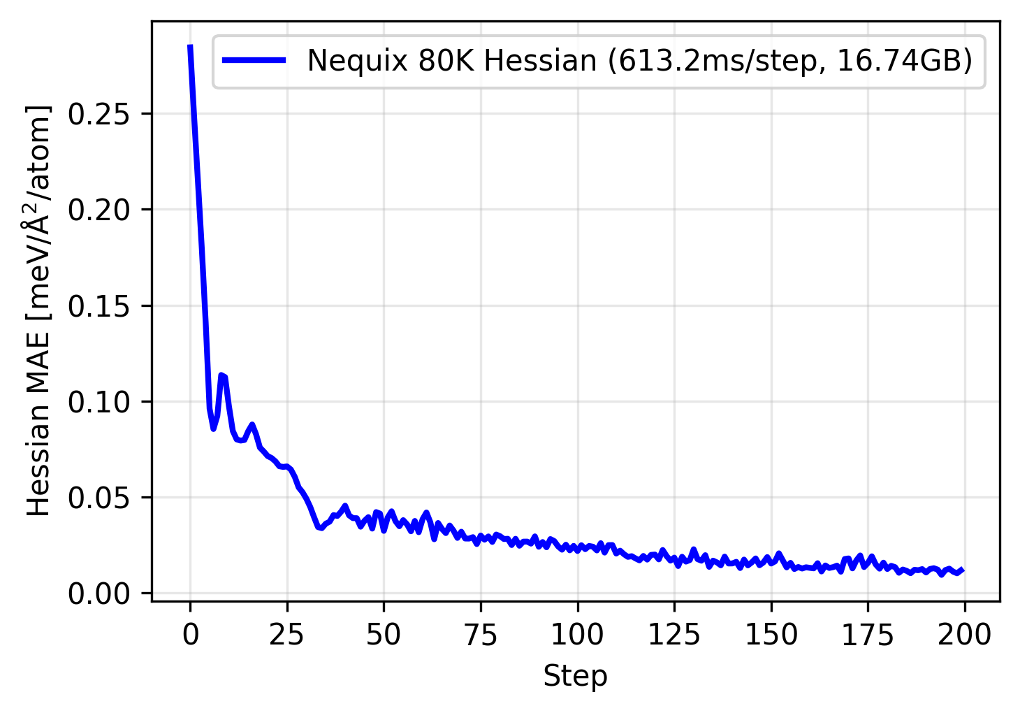
The model trains nicely, however even this 80 thousand parameter model on a single material uses over 16 gigabyte of memory, and also quite slow at over 600 milliseconds per step. Since the Hessian computation scales $O(N^2)$ in time and space complexity with respect to the number of atoms, this becomes prohibitively expensive for any larger materials or batch sizes larger than one, even on the largest commercially available GPUs. Furthermore, scaling the model to sizes of current universal MLIPs, often in the million to even billion parameter range is impossible.
Stochastic Hessian-vector product
One trick we can use to greatly improve the efficiency of training is to instead train on randomly sampled columns of the Hessian. This involves randomly selecting one atom $b$ and Cartesian direction $j$, selecting only those indices of the force constants in the computation of the loss. This results in a force constant loss $\mathcal{L}_\Phi$ of:
\[\mathcal{L}_\Phi = \frac{1}{3 N_a} \sum_{a=1}^{N_a} \sum_{i=1}^{3} \mathbb{E}_{\substack{b \sim \mathcal{U}[1,N_a] \\ j \sim \mathcal{U}[1,3]}} \left| \frac{\partial^2 \hat{E}}{\partial r_{a,i} \, \partial r_{b,j}} - \Phi_{aibj} \right|\\\]The column of the Hessian can be computed with a Hessian-vector product (HVP), where
the vector is an indicator vector of all zeros with a one at the index
corresponding to the selected atom and Cartesian direction. The HVP can be
computed efficiently in $O(N)$ time and space complexity, without computing or
materializing the full Hessian. In practice this can be done using a
forward-mode Jacobian-vector product (jax.jvp or torch.func.jvp) over the
reverse mode gradient.
We implement this into our code below, replacing the old full Hessian training.
 def train(model, graph, ref_hessian, n_epochs=200, lr=0.003):
     def energy_fn(model, pos_flat):
         pos = pos_flat.reshape(graph["positions"].shape)
         offset = graph["shifts"] @ graph["cell"]
         disp = pos[graph["senders"]] - pos[graph["receivers"]] + offset
         return model.node_energies(
             disp, graph["species"], graph["senders"], graph["receivers"]
         ).sum()

     grad_fn = jax.grad(energy_fn, argnums=1)

-    def hessian_fn(model, x):
-        return jax.jacfwd(lambda pos: grad_fn(model, pos))(x)
+    def hvp_fn(model, x, v):
+        return jax.jvp(lambda pos: grad_fn(model, pos), (x,), (v,))[1]

     optimizer = optax.adam(lr)
     opt_state = optimizer.init(eqx.filter(model, eqx.is_array))

     @eqx.filter_jit
-    def train_step(model, opt_state, pos_flat):
+    def train_step(model, opt_state, pos_flat, idx):
         def loss_fn(model):
-            hessian = hessian_fn(model, pos_flat)
-            return jnp.abs(hessian - ref_hessian).mean()
+            v = jnp.zeros_like(pos_flat).at[idx].set(1.0)
+            hvp = hvp_fn(model, pos_flat, v)
+            return jnp.abs(hvp - ref_hessian[:, idx]).mean()

         loss, grads = eqx.filter_value_and_grad(loss_fn)(model)
         updates, opt_state_new = optimizer.update(grads, opt_state, model)
         model = eqx.apply_updates(model, updates)
         return model, opt_state_new, loss

     pos_flat = graph["positions"].flatten()
     losses = []
+    rng_key = jax.random.key(0)
     for epoch in tqdm(range(n_epochs)):
-        model, opt_state, loss = train_step(model, opt_state, pos_flat)
+        rng_key, subkey = jax.random.split(rng_key)
+        idx = jax.random.randint(subkey, (), 0, pos_flat.shape[0])
+        model, opt_state, loss = train_step(model, opt_state, pos_flat, idx)
         losses.append(float(loss))

     return losses
 def train(model, graph, ref_hessian, n_epochs=200, lr=0.003):
     def energy_fn(pos_flat):
         pos = pos_flat.view(*graph["positions"].shape)
         offset = graph["shifts"] @ graph["cell"]
         disp = pos[graph["senders"]] - pos[graph["receivers"]] + offset
         return model.node_energies(
             disp, graph["species"], graph["senders"], graph["receivers"]
         ).sum()

     grad_fn = torch.func.grad(energy_fn)
-    hessian_fn = torch.compile(torch.func.jacfwd(grad_fn))
+    hvp_fn = torch.compile(lambda x, v: torch.func.jvp(grad_fn, (x,), (v,))[1])

     pos_flat = graph["positions"].flatten()
     losses = []
     optimizer = torch.optim.Adam(model.parameters(), lr=lr)


     for epoch in tqdm(range(n_epochs)):
         optimizer.zero_grad()
-        hessian = hessian_fn(pos_flat)
-        loss = (hessian - ref_hessian).abs().mean()
+        idx = torch.randint(pos_flat.shape[0], (1,), device=device).item()
+        v = torch.zeros_like(pos_flat)
+        v[idx] = 1.0
+        hvp = hvp_fn(pos_flat, v)
+        loss = (hvp - ref_hessian[:, idx]).abs().mean()
         loss.backward()
         optimizer.step()
         losses.append(loss.item())

     return losses
Once again, we can use this to train our tiny 80 thousand parameter model:
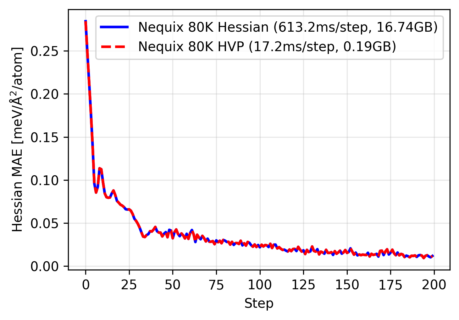
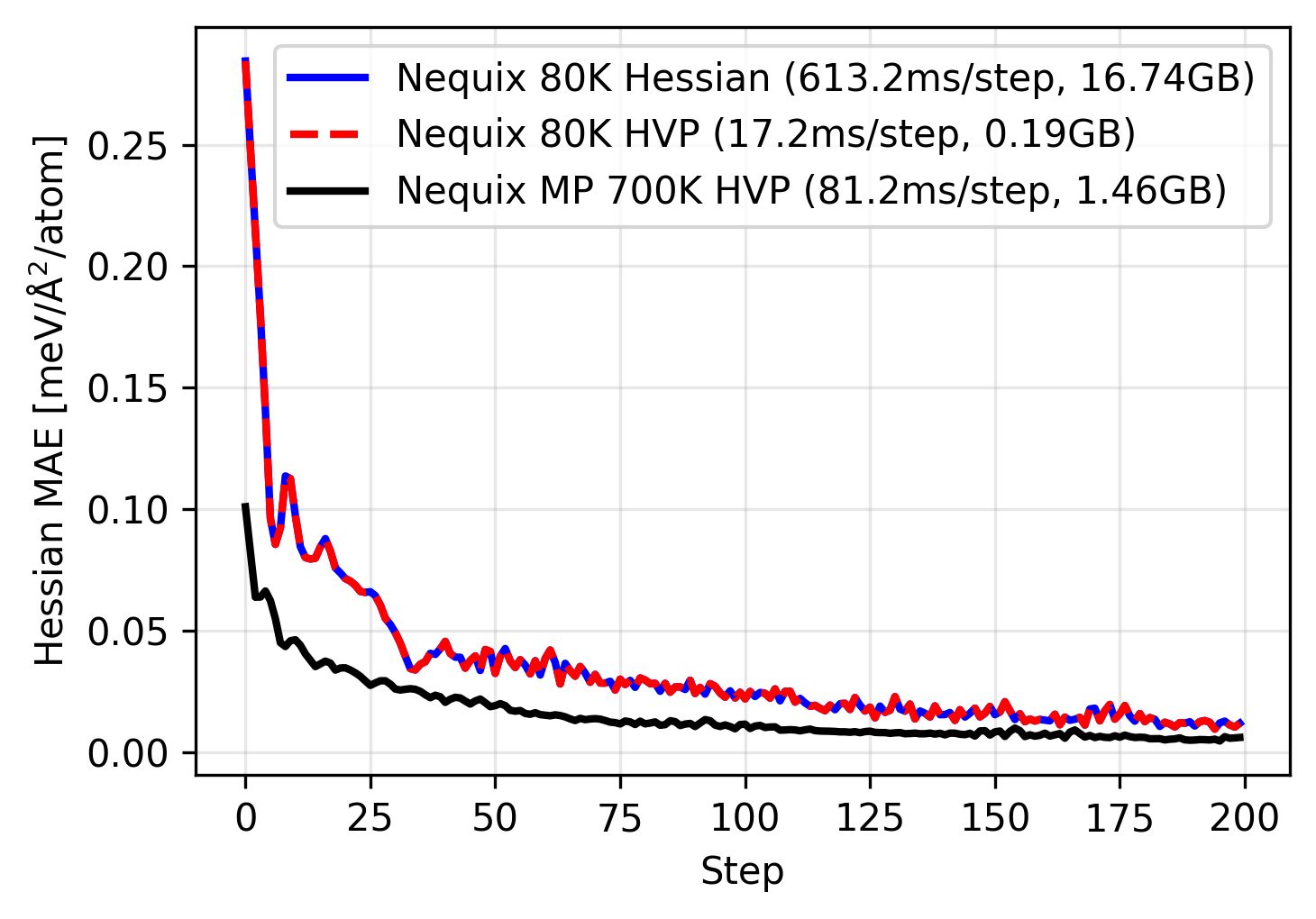
This time we see that the training trajectory follows the same path as the full Hessian training, however it is over 35 times faster and using over 80 times less memory. Since the HVP scales linearly with respect to number of atoms, this also lets us run on much larger systems, or parallelize across larger batch sizes.
Why does the HVP training match the full Hessian exactly? This is due to symmetry. The Silicon primitive cell has two symmetrically equivalent atoms, which means a single column of the Hessian (even for the 64-atom supercell) contains sufficient information for the full Hessian. This also explains the patterns we see in the visualization of the force constants above. Since we are using an E(3)-equivariant neural network, the model can be trained on one column and predict all other columns correctly by design! This is not always the case, although most materials exhibit symmetries that greatly reduce number of elements in the Hessian that would need to be sampled. For more on this see the paper.
Fine-tuning universal MLIPs
With efficient force constant training implemented, we can set out to accomplish our original goal: fine-tuning a universal MLIP on phonon calculations. To illustrate this, we can load the Nequix MP, a competitive 700 thousand parameter model trained on over 1 million DFT calculations from Materials Project, and fine-tune it on our Silicon force constants:
calc = NequixCalculator("nequix-mp-1")
model = calc.model
graph = preprocess_graph(atoms, calc.atom_indices, calc.cutoff, targets=False)
train(model, graph, ref_hessian, lr=0.0001)
calc = NequixCalculator("nequix-mp-1", backend="torch", use_kernel=False)
model = calc.model.to(device)
model.train()
g = preprocess_graph(atoms, calc.atom_indices, calc.cutoff, targets=False)
graph = {
    k: torch.as_tensor(
        v, device=device, dtype=torch.float32 if v.dtype == np.float32 else torch.long
    )
    for k, v in g.items()
}
train(model, graph, ref_hessian, lr=0.0001)
We find the full model can be fine-tuned quickly with a small amount of memory. This enables us to fine-tune the model on a full database of phonon calculations. We also observe the benefit of pretraining: the model starts out with a significantly lower Hessian error and can reach an even lower error during training. While overfitting to a single example is not the best demonstration of this, we find that pretrained models already exhibit good Hessian errors, yet phonon fine-tuning can improve them further.
PFT Results
Using the method above, we fine-tune the Nequix MP model on the MDR Phonon database which was recalculated using the same DFT settings at Materials Project and made available at Alexandria (Loew et al., 2025). These calculations are performed on a subset of the materials within Materials Project, so the model is not shown any new geometries or chemistries; the only additional data is from the force constants. For the full PFT method, we train on a multi-objective loss consisting of energy, force, stress, and the force-constant term discussed above:
\[\mathcal{L}_\text{PFT} = \lambda_E\mathcal{L}_E + \lambda_F\mathcal{L}_F + \lambda_\sigma\mathcal{L}_\sigma + \lambda_\Phi\mathcal{L}_\Phi\]In the paper we also discuss a co-training procedure which is necessary to prevent catastrophic forgetting of the potential energy surface.
Phonon properties
Evaluating the model on held-out phonon data, we demonstrate that PFT results in an average 55% reduction in mean absolute error (MAE) of several phonon properties from the base Nequix MP model, and is state-of-the-art among models trained on Materials Project structures:
Table: Evaluation of models on held-out MDR Phonon data. Metrics are MAE of maximum phonon frequency $\omega_{\max}$ (K), vibrational entropy $S$ (J/K/mol), Helmholtz free energy $F$ (kJ/mol) and heat capacity at constant volume $C_V$ (J/K/mol).
| Model | $\omega_{\max}$ | $S$ | $F$ | $C_V$ |
|---|---|---|---|---|
| MACE-MP-0 | 61 | 60 | 24 | 13 |
| SevenNet-0 | 38 | 47 | 18 | 8 |
| Nequix MP | 24 | 32 | 12 | 6 |
| SevenNet-l3i5 | 25 | 25 | 9 | 4 |
| eSEN-MP | 24 | 14 | 4 | 5 |
| Nequix MP PFT | 12 | 14 | 5 | 3 |
| Nequix MP PFT (no cotrain) | 10 | 11 | 4 | 2 |
Remarkably, the MP PFT model also outperforms the Nequix OAM model trained on OMat24 and sAlex, which has $\omega_{\max}$/$S$/$F$/$C_V$ MAE of 17/18/7/4 respectively, despite the PFT model being trained with approximately two orders of magnitude fewer DFT calculations. This suggests that PFT can be more data efficient for achieving accurate phonon properties.
Thermal conductivity
In addition, we demonstrate that PFT generalizes to improved performance on thermal conductivity predictions, which are computed from third-order force constants (i.e. the third derivative of energy). We observe a 31% improvement in thermal conductivity prediction error from the base model, and again show state-of-the-art performance among models trained on Materials Project; all with a significantly smaller and faster model.
Table: Matbench Discovery “compliant” leaderboard for thermal conductivity, measured in symmetric relative mean error in predicted phonon mode contributions to thermal conductivity $\kappa_{\mathrm{SRME}}$.
| Model | Params | $\kappa_{\mathrm{SRME}} \downarrow$ |
|---|---|---|
| ORB v2 MPtrj | 25.2M | 1.725 |
| eqV2 S DeNS | 31.2M | 1.676 |
| MatRIS v0.5.0 MPtrj | 5.83M | 0.865 |
| MACE-MP-0 | 4.69M | 0.682 |
| DPA-3.1-MPtrj | 4.81M | 0.650 |
| HIENet | 7.51M | 0.642 |
| SevenNet-l3i5 | 1.17M | 0.550 |
| GRACE-2L-MPtrj | 15.3M | 0.525 |
| Nequip-MP-L | 9.6M | 0.452 |
| Nequix MP | 707K | 0.446 |
| Eqnorm MPtrj | 1.31M | 0.408 |
| eSEN-30M-MP | 30.1M | 0.340 |
| Nequix MP PFT | 707K | 0.307 |
| Nequix MP PFT (no cotrain) | 707K | 0.281 |
Conclusion
Phonon fine-tuning is simple, model agnostic method to improve vibrational and thermal property prediction by training directly on force constants. It is important to note that training requires access to higher-order derivatives, which may not be accessible for all universal models. For more for information about the method and additional results, including those for the OAM model, see the full paper.
If you found the paper or blog post useful in your research, please cite with:
@article{koker2026pft,
  title={{PFT}: Phonon Fine-tuning for Machine Learned Interatomic Potentials},
  author={Koker, Teddy and Gangan, Abhijeet and Kotak, Mit and Marian, Jaime and Smidt, Tess},
  journal={arXiv preprint arXiv:2601.07742},
  year={2026}
}
- Loew, A., Sun, D., Wang, H.-C., Botti, S., & Marques, M. A. L. (2025). Universal machine learning interatomic potentials are ready for phonons. Npj Computational Materials, 11(1), 178.
- Koker, T., Kotak, M., & Smidt, T. (2025). Training a Foundation Model for Materials on a Budget. ArXiv Preprint ArXiv:2508.16067.